Tidy3D
Case studies
Choose the category you are interested in:

Renowned photonics researcher and Stanford professor honored for pioneering work in computational electromagnetics and nanophotonics
[Boston, April 30, 2025] – Flexcompute proudly congratulates Dr. Shanhui Fan, co-founder of Flexcompute and a world-renowned expert in photonics and electromagnetism, on his election to the U.S. National Academy of Sciences (NAS), one of the highest honors in American science.
Dr. Fan is a professor of electrical engineering and applied physics at Stanford University and has played a pivotal role in shaping the theoretical and computational foundations of modern photonics. His research spans nanophotonics, photonic crystals, metamaterials, plasmonics and solar energy conversion, with a strong emphasis on computational methods, a core strength that he brought to Flexcompute.
As co-founder of Flexcompute, Dr. Fan helped establish the company’s mission to revolutionize scientific computing, delivering breakthrough simulation performance for electromagnetics, fluid dynamics and beyond. His vision continues to drive Flexcompute’s innovation at the intersection of physics and high-performance computing.
Dr. Fan earned his Ph.D. from the Massachusetts Institute of Technology under the mentorship of John Joannopoulos. With an h-index of 177, he is one of the most highly cited researchers in his field.
“Shanhui’s election into the National Academy of Sciences is not only a recognition of his extraordinary scientific achievements, but also a validation of the deep scientific principles that guide our work at Flexcompute,” said Vera Yang, Flexcompute Co-Founder and President. “We’re honored to have him as a co-founder and collaborator.”
Dr. Fan is one of 120 new U.S-based members elected in 2025 for distinguished and continuing achievements in original research. For more information on the NAS 2025 elections, visit nasonline.org.
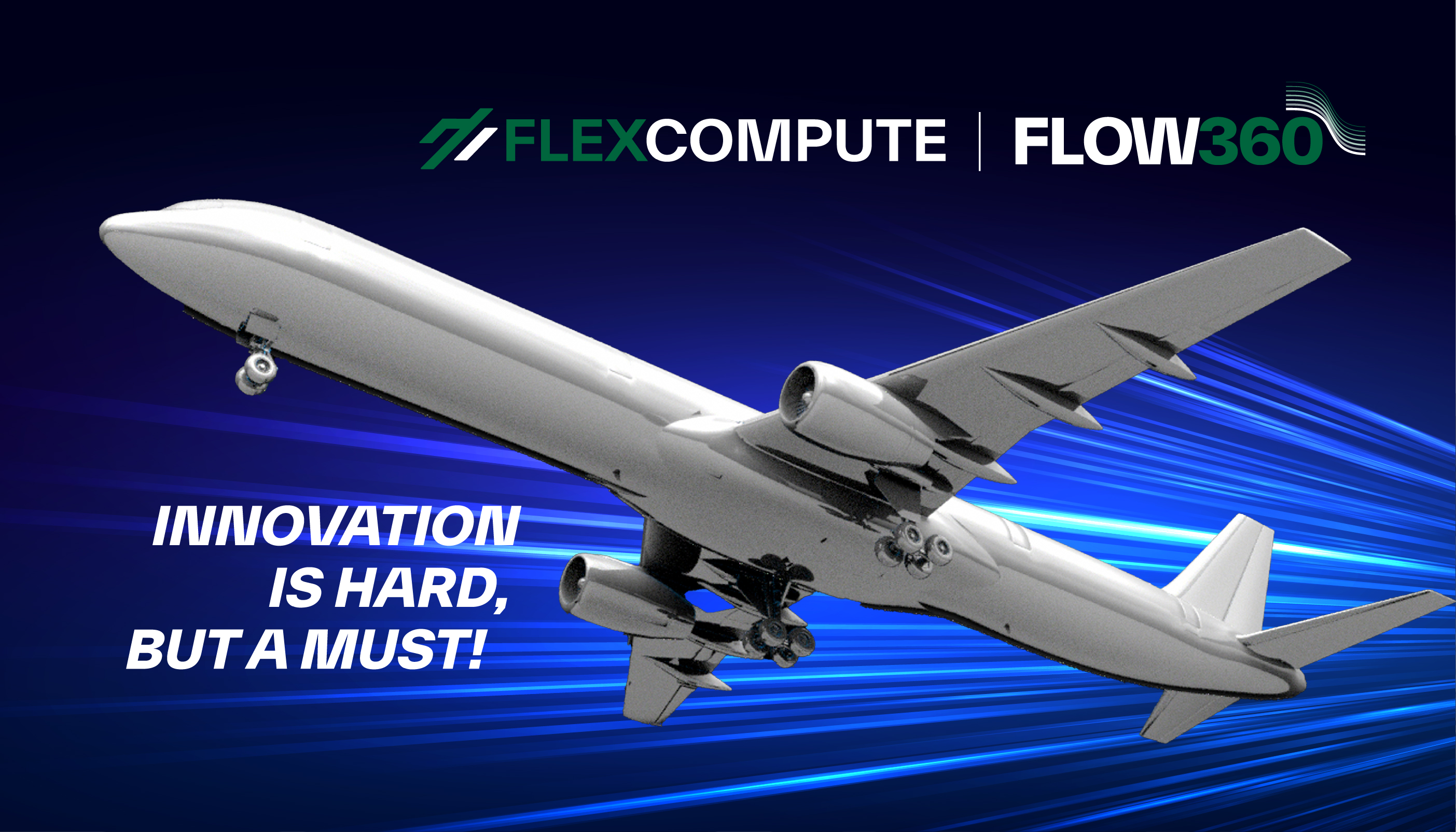
Innovation is hard, but it’s non-negotiable.
At Flexcompute, we just celebrated 10 years of leading innovation in physics simulation. It’s been an exhilarating journey: assembling a team of the brightest minds, building a full-stack software-hardware architecture for modern GPUs, designing algorithms from scratch, and cutting simulation time without sacrificing accuracy.
Starting with a revolutionary idea is one thing.
Pushing beyond it, again and again, at startup speed is where true innovation lives.
Our mission is simple: make hardware innovation as easy as software innovation.
That’s why we built Flow360, the world’s first GPU-native Computational Fluid Dynamics (CFD) solver, delivering 10–100 times faster performance than traditional CPU-based tools.
But we didn’t stop there.
Flow360 is not just fast, it keeps getting faster.
Speeding Up What’s Already Fast
By late 2022, most obvious speed-up opportunities had already been captured. Improving beyond that point wasn’t easy. It demanded deep innovation and smarter, more adaptive methods.
Yet, over the past two years, the Flexcompute team pushed even harder, making Flow360 significantly faster once again.
Here’s what we achieved:
Real-World Performance: 3X Faster in Two Years on Same Hardware
Geometry and Simulation Setup:
We used a typical aerospace configuration of an aircraft with fuselage, wings, horizontal and vertical tails, and propeller booms meshed automatically by Flow360 (~25 million nodes).
Simulations were run at Mach 0.15 and 2 degrees angle of attack (AoA), consistently across two years of solver versions.

Figure 1: Flow visualization over the aircraft with skin friction vectors.
Convergence Efficiency:
A fair comparison was maintained: convergence was defined when lift (CL) and drag (CD) changed less than 0.05% across 500 pseudo steps.
Results:
-
January 2023: 4,900 pseudo steps to converge
-
February 2025: 1,600 pseudo steps to converge
A massive 3 times reduction in steps, without compromising accuracy.

Figure 2: Convergence of CL and CD across solver releases from last 2 years.
Runtime Efficiency:
All tests were performed on identical hardware (8× A100 GPUs).
-
January 2023: ~10 minutes total runtime
- February 2025: 3.2 minutes total runtime

Figure 3: Evolution of runtime across solver releases from last 2 years.
Even in early 2023, Flow360 was already setting a new standard, simulating a 25-million-node mesh with a stringent convergence criterion in just 10 minutes.
In contrast, traditional CPU-based CFD tools would take several hours to complete a similar case providing a 100X speed advantage.
Today, with the latest release, Flow360 cuts that time down even further to just 3.2 minutes on the same hardware. Another 3X improvement in just two years.
How We Made Flow360 Even Faster
The speed-up didn’t come from shortcuts. It came from smarter, more robust techniques, each rigorously tested across a wide range of cases before every release.
Smarter Time-Stepping: Adaptive CFL
In early 2023, Flow360 used a traditional Ramp CFL method requiring users to manually set CFL values. Set it too aggressively, and simulations could diverge. Set it too conservatively, and convergence dragged painfully slow.
We eliminated this trade-off by introducing Adaptive CFL, an automatic system that dynamically adjusts CFL based on real-time solver behavior. Now, the solver accelerates convergence while guarding against instability with no manual tuning needed.
Expanded Solver Robustness
Throughout 2023, we continually strengthened Flow360’s performance across a wider range of cases. Even with only a minor increase in runtime, solver reliability and accuracy improved dramatically.
Major Leap: Low-Mach Preconditioning
In mid-2024, we implemented Low-Mach Preconditioning, boosting convergence and accuracy for low-speed flows critical to:
- Take-off and landing of commercial aircraft
- VTOL hovering operations
- Automotive aerodynamics simulations
The result: faster convergence and lower runtimes across key real-world applications.
Streamlined WebUI: End-to-End Workflow
In late 2024, we overhauled the WebUI, consolidating geometry, meshing, and case management into a single unified project workspace. The upgrade drastically simplified workflows and cut setup time.
Pushing Limits: Smart CFL-Cut
In early 2025, we pushed Adaptive CFL even further by introducing Smart CFL-Cut. If instability is detected, Flow360 automatically trims CFL values, allowing users to run simulations more aggressively, without risking divergence.
The result?
Every innovation compounds.
Every release moves faster, smarter, and more reliably which sets a new standard for GPU-native simulation.
Why It Matters for Customers
Every breakthrough in speed directly translates to lower simulation costs.
When your case converges in 3 times fewer pseudo steps, you pay 3 times less, without any compromise in accuracy or reliability.
Faster, cheaper simulations mean you can:
- Explore broader design spaces with greater confidence
- Evaluate more flight conditions to capture edge cases earlier
- Build more comprehensive aerodynamic databases which reduces risk in later-stage testing
- Run large-scale, high-fidelity simulations that better replicate real-world conditions
- Accelerate product development and get to market faster
Innovation isn’t just happening behind the scenes, it’s happening for you, in every simulation, every decision, and every breakthrough.
What’s Next?
Hold on tight, we’re just getting started. Our team is already charging full-speed into the next wave of breakthroughs:
- We’re boosting even faster solver speeds, especially for aeroacoustics simulations and unsteady high-fidelity runs, so time-to-solution will never slow down your innovation again.
- We’re ramping up mesh generation speed by an entire order of magnitude. Imagine starting a hundred-million-point unstructured simulation in minutes instead of hours.
- But we’re taking it even further, streamlining the earliest stages of your analysis workflow, geometry handling, so those gnarly, “dirty” CAD models become simulation-ready in minutes, not days of grunt work!
- Plus, our upcoming adaptive meshing and intelligent geometry technologies take the grind out of the process, automatically optimizing for the highest accuracy at the fastest turnaround.
Stay tuned. At Flexcompute, we don’t just keep pace with innovation. We set it.
Ready to move faster than ever before?
Contact us to learn how Flow360 can transform your engineering workflows.

Introduction
In 2024, Flexcompute participated in the AutoCFD4 workshop, where we presented our highly accurate and fast results for the DrivAer model. The AutoCFD4 workshop is an international forum for researchers and practitioners in the field of automotive Computational Fluid Dynamics (CFD). The workshop provides a platform for the exchange of ideas and experiences on the latest developments in automotive CFD.
DrivAer Model
The AutoCFD4 workshop focuses on two test cases: the Windsor model and the DrivAer model. However, it’s the DrivAer model that generally garners more attention, primarily because it’s a reasonably accurate representation of a real-life commercial car It is a complex geometry that is used to benchmark the accuracy and efficiency of CFD solvers. While the geometry, boundary condition, and computation grid are provided by the committee, the workshop offers interesting insights into various turbulence models and numerical schemes.

Speed and Accuracy of Flow360
Traditional CFD tools require days or even weeks to perform a simulation of an automotive geometry. In contrast, Flow360 requires only 10-15 min for a RANS simulation and 1-2 hours for a DDES simulation of the DrivAer model with the committee-provided grid. With this speed, CFD engineers working on Formula 1, commercial cars, or sports cars no longer need to wait for lengthy periods to evaluate design changes. Design iterations can be done at a much faster pace, with the advantage of high accuracy of DDES simulations. Flow360’s accuracy aids automotive companies in making informed design decisions, while its speed significantly reduces time for design cycles, resulting in faster time-to-market.

A comparison of Flow360’s DDES results for the DrivAer model with the test performed in the Pininfarina wind tunnel shown above highlights the capability of Flow360. For a CFD tool to be used in the rigorous design and optimization of automotive, it’s essential to capture complex flow features including corner flow, origin and evolutions of vortices, and tiny wake structures. Without this capability, it is challenging to determine whether a marginal design change is acceptable or not. Flow360’s accuracy with the combination of speed exactly addresses this concern by providing an efficient solution.
Conclusion
Flow360’s remarkable speed, coupled with the high accuracy of its results, showcases its potential to revolutionize automotive CFD workflows. We invite you to experience the Flow360 advantage today. Talk to an expert to learn more about Flow360.

“In our pursuit of excellence, we don’t compromise one aspect to enhance another.” – Qiqi Wang, Co-founder of Flexcompute and architect of Flow360
At Flexcompute, we live by this philosophy. During the Automotive CFD Prediction Workshop (AutoCFD4), Flow360 showcased its exceptional ability to deliver world class speed and accuracy—simultaneously.
AutoCFD is an international forum that brings together leading OEMs, universities, and CFD practitioners to benchmark simulations against wind tunnel data on standardized automotive geometries. It’s a proving ground—and Flow360 delivered.
While we’re proud to offer the fastest solver (see below), our mission goes beyond speed. Flow360 is an end-to-end platform that automates the tedious parts of simulation—geometry cleanup, meshing, setup, and reporting—so engineers can focus on what matters: innovation.
Benchmarking Flow360 on the DrivAer Model
We focused on the DrivAer model, a highly detailed and realistic geometry widely adopted for CFD benchmarking. Provided by the workshop committee, the standardized geometry, boundary conditions, and mesh ensure a level playing field. With comprehensive validation data—pressure taps, velocity probes, and PIV imagery—the DrivAer model is a rigorous testbed, and Flow360 passed with flying colors.
DrivAer Model
 |
| Figure 1: Visualization of an isosurface of Q-criterion for DrivAer model |
Fast, Automated Meshing
Flow360 includes a powerful, feature-rich meshing tool. For AutoCFD4, it generated a hex-dominant mesh with 145 million nodes in just 60 minutes. This meshing workflow is easily automated using our Python API, enabling seamless integration into streamlined engineering pipelines.
 |
 |
| Figure 2: Visualization of the mesh for the DrivAer model generated with Flow360’s meshing tool | |
RANS Predictions by the Time You Finish Your Coffee (10 Min)
Traditional CFD tools take days to simulate realistic automotive geometries. Flow360 changes the game.
We completed a full RANS simulation of the DrivAer model in just 10 minutes on 48 A100 GPUs—without compromising accuracy. This was made possible by:
- A blended central/upwind scheme to reduce numerical viscosity
- A low Mach number preconditioner to enhance convergence
- An adaptive CFL strategy for stability and robustness
- User control over turbulence model coefficients, including an α₁ adjustment in the K-ω SST model (set to 0.4 to better capture separation over the roof)
The integrated force predictions from Flow360 showed excellent agreement with physical test data, with just 2 drag counts of difference—a level of accuracy rarely seen at this speed.

Figure 3: Comparison of integrated forces between Flow360 RANS and Test data having only 2 drag count difference
Scale-Resolved Simulation by the Time You Finish Lunch (37 min)
As OEMs increasingly adopt transient simulations for greater accuracy and faster design cycles, Flow360 continues to push boundaries. One major leap: support for Zonal Detached Eddy Simulation (ZDES) using the Deck-Renard shielding function, enhancing separation prediction in critical flow regions.
For AutoCFD4, we submitted a ZDES simulation using this approach. Total wall time: just 37 minutes, including both phases below:
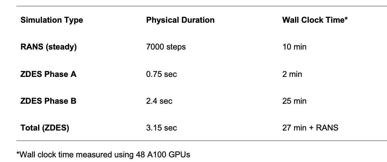
Table 1: Simulation Timing Summary | *Wall clock time measured using 48 A100 GPUs
This two-phase ZDES approach done automatically in sequence with adaptive time-stepping:
- A coarse time step (5e-3 s, CFL = 50 on a resolved mesh zone) to flush the RANS solution for 0.75 sec—completed in 2 minutes on 48 A200 GPUs
- A fine time step (1e-3 s, CFL = 10) for the main ZDES run, averaged over the last 2 seconds—completed in 25 minutes on 48 A100 GPUs
All of this, without sacrificing fidelity. Flow360’s ZDES results match physical testing within 1 drag count, capturing complex flow physics that engineers can trust.

Figure 8: Flow360 ZDES’s excellent prediction of delta forces prediction between two DrivAer configurations with the Test data
Right Answers for the Right Reasons
Physically accurate flow features are essential for design optimization. Many CFD tools struggle to resolve complex flow phenomena, particularly around critical regions like the A-pillar and side mirror, where flow separation and downstream vortices significantly impact the pressure distribution on the side window. Flow360’s ZDES results, however, show close agreement with test data, validating its ability to capture the true physics of the flow.
 |
 |
 |
This high level of accuracy continues along the symmetry plane of both the upper body and underbody, where Flow360’s pressure predictions align closely with wind tunnel data. Such consistency reinforces trust in the solver’s reliability for production use.
 |
 |
Even in the most challenging regions—such as the rear wake and underfloor—Flow360 delivers. The wake contours show excellent agreement with test results, clearly demonstrating that Flow360 captures not just trends, but the detailed unsteady structures that matter most to real-world aerodynamic performance.

Figure 5: Visualization of flow structure around A-piller and side mirror along with excellent agreement between Flow360 and Test data for pressure prediction on side mirror
Delta Prediction: Where It Counts in Design Optimization
In the production stage, the priority shifts from absolute accuracy to capturing aerodynamic deltas—the impact of design changes on performance. At this point, vehicle designs are largely frozen, and the focus shifts to fine-tuning specific components—such as mirrors, underbody panels, or wheel deflectors—to optimize efficiency. What matters most is the ability to reliably capture how each design tweak impacts overall drag performance.
One of AutoCFD4’s most important test cases was the front wheel arch deflector delta—a highly relevant real-world scenario given how often such features are refined late in the design cycle.

Figure 8: Flow360 ZDES’s excellent prediction of delta forces prediction between two DrivAer configurations with the Test data
Flow360 accurately captured both the magnitude and trend of the delta, enabling confident decision-making and reducing reliance on costly wind tunnel validation. It’s precisely why Flow360 is already trusted in production by leading automotive OEMs.
Real-World Validation: NIO Success Story
Flow360 isn’t just proven in benchmarks—it’s trusted in production. In collaboration with NIO Inc., we validated over 60 designs across SUVs and sedans. The results:
- Fastest Speed and Efficiency: Flow360’s simulation time is 10-100 times faster than traditional methods, completing complex simulations in just an hour on 8 L20 (10 mins on 8 H200)
- Unparalleled Accuracy: More than 94% of simulations show less than 3% deviation from physical wind tunnel tests, ensuring that design decisions are based on reliable data.
Many tools struggle in robustness and consistency across extensive test scenarios —Flow360 delivers.
In the example below Flow360 accurately captured the design delta Cd caused by a small change to air-intake. This was particularly challenging as it is located near the wheel well. With Flow360 you can have confidence in your results to make the right decisions.

Figure 9: Accurate prediction of delta Cd by Flow360 as compared to a competitor for a design change due to air-intake
And the Best Part? We’re Just Getting Started
Flow360 combines unmatched solver speed with high-fidelity results—redefining how automotive CFD gets done. But this is just the beginning.
Behind Flow360 is a world-class team shaping the future of simulation. We’re proud to be working with some of the most respected minds in the field—like Dr. Philippe Spalart, the pioneer behind the Spalart-Allmaras turbulence model; Dr. Mike Park, former NASA researcher and global leader in adaptive mesh refinement; and Dr. Roberto Della Ratta Rinaldi, former senior aerodynamicist at Aston Martin and McLaren, with over 15 years at the forefront of automotive aero analysis and methodology development.
Together, this team isn’t just evolving CFD—they’re accelerating it beyond anything the industry has seen. Flow360 enables interactive workflows at unprecedented speed, taking engineers from geometry to insight in hours, not days.
And there’s more ahead. In Q3 2025, we’ll be launching a major release focused on geometry, further simplifying simulation and introducing new levels of automation and intelligence into the workflow.
If you’re building the future, choose a partner that represents the future.
Experience Flow360—and see how fast innovation can move. Talk to an expert to learn more about Flow360.

Flexcompute Partners with Samsung Display to Advance Optical Simulation in Display Technology
We are excited to announce a groundbreaking partnership between Flexcompute and Samsung Display. As a global leader in advanced display technologies, Samsung Display has chosen Tidy3D, Flexcompute’s flagship electromagnetic simulation platform, to power its next-generation optical display simulations and analyses.

A New Era in Display Innovation
With display technologies becoming increasingly complex and performance-driven, the need for fast, accurate, and multi-physics simulation tools has never been greater. Tidy3D rises to this challenge with its GPU-accelerated architecture, delivering exceptional computational speed without compromising on accuracy. The platform supports a wide range of simulation capabilities that are essential for modeling advanced display structures—from thin-film interference to light extraction and beyond.
Samsung Display’s decision to integrate Tidy3D into their workflow reflects the platform’s ability to meet the highest standards of industrial R&D. Whether it’s evaluating electromagnetic behavior, optimizing light propagation, or ensuring compatibility with multi-physics requirements, Tidy3D enables rapid, detailed insights into complex optical systems.
Why Tidy3D?
Tidy3D is built for performance and precision. It allows researchers and engineers to:
- Run simulations in a fraction of the time required by traditional FDTD solvers, allowing you to publish faster and increase your research output.
- With the native integration of PhotonForge, the unified platform for fabrication-aware photonic design, with Tidy3D, one can design photonic circuits, simulate performance, and generate fabrication-ready layouts — all within a streamlined workflow.
- Incorporate material models and boundary conditions for accurate physical representation.
- Conduct parametric sweeps and optimizations with minimal setup.
- Leverage adjoint-based inverse design for innovative device geometries.
These features are expected to play a critical role in keeping Samsung Display at the forefront of display technology by accelerating innovation through high-performance computing.
Looking Ahead
This partnership not only validates the capabilities of Tidy3D but also signifies a broader movement toward simulation-driven innovation in consumer electronics. Flexcompute is proud to support Samsung Display’s continued innovation, and is committed to empowering engineers and scientists with the tools they need to push the boundaries of what’s possible in display design.
As we move forward, we look forward to sharing more updates on how Tidy3D is being used to develop the next generation of visual experiences.
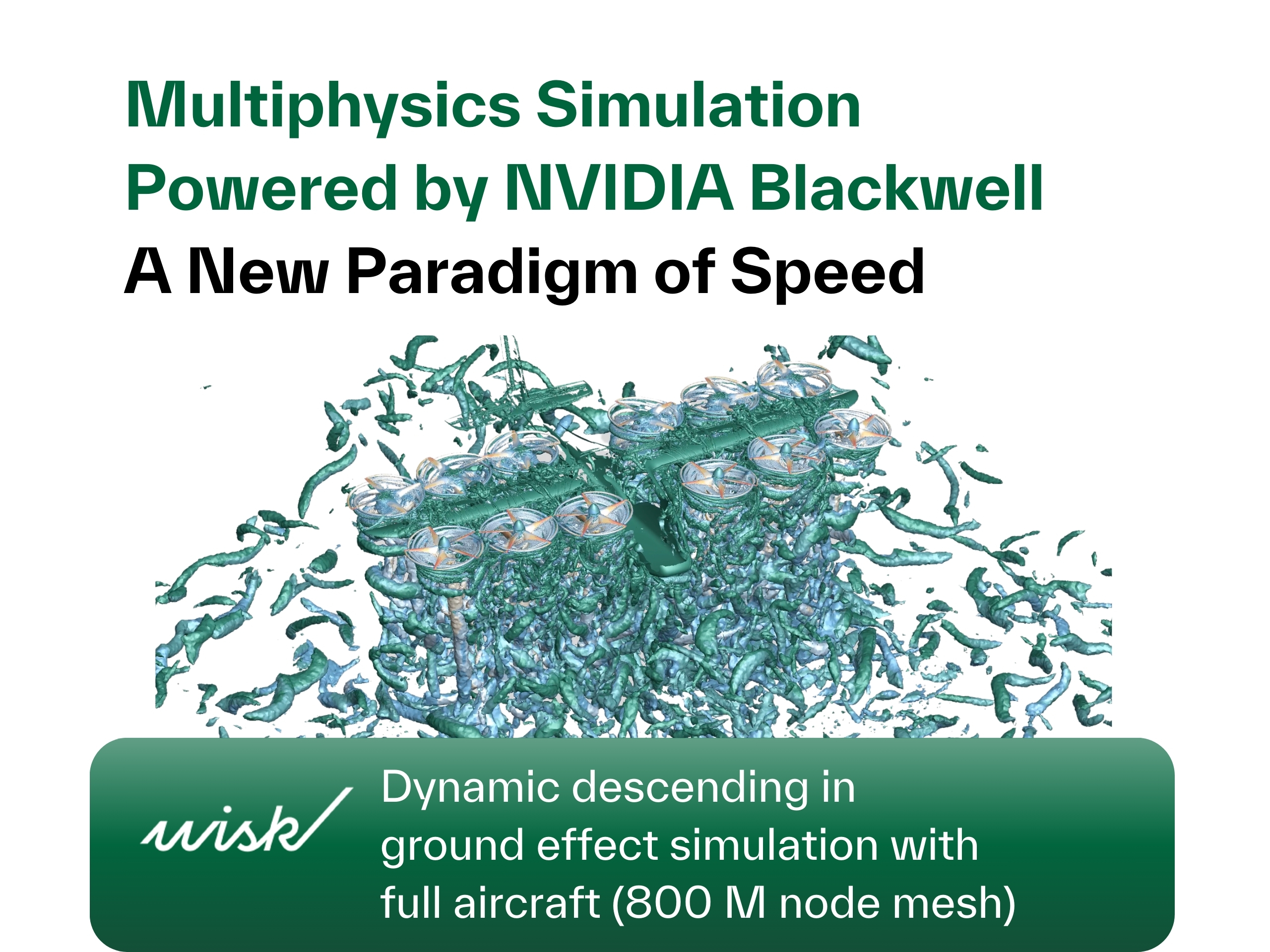
Flexcompute Unveils High-Fidelity Physics Simulation Powered by NVIDIA Blackwell Platform for a New Paradigm of Speed
Innovative companies including Beta Technologies, Celestial AI, Dufour Aerospace, JetZero, Joby Aviation, and Kyocera SLD Laser, Inc. adopt Flexcompute powered by NVIDIA Blackwell
[Boston, March 18, 2025] – Flexcompute, the leading provider of multi-physics simulation technology, announced support for the NVIDIA Blackwell platform, marking the dawn of a new era in simulation capabilities. As a GPU-native, high-fidelity solution already known for being 100 times faster than leading simulation technologies, Flexcompute products powered by Blackwell will enable its customers to conduct high-fidelity physics simulations faster than ever before.
“We are thrilled to offer our customers early access to our products accelerated by NVIDIA Blackwell GPUs,” said Vera Yang, President of Flexcompute. “Leveraging NVIDIA’s cutting-edge GPU technology to Flexcompute’s industry-leading simulation platform, we are enabling engineers to solve complex real-world problems faster and more accurately than ever before. This collaboration marks a new era of simulation-driven innovation, where design cycles are accelerated, and breakthroughs become reality.”
“NVIDIA Blackwell is powering a new era of computing, delivering exceptional performance for the most demanding applications. Flexcompute’s adoption of Blackwell enables industries to tap into the full potential of this revolutionary technology, transforming the way simulations are created and accelerating the path from concept to reality,” Tim Costa, senior director for CAE and CUDA-X at NVIDIA said.
Some of the most innovative companies in aerospace, automotive, electronics, and technology are already leveraging Flexcompute’s simulation technology powered by NVIDIA Blackwell including Beta Technologies, Celestial AI, Dufour Aerospace, JetZero, Joby Aviation, Kyocera SLD Laser, Inc., and more. Customer use cases include:
- Beta Technologies leverages Flow360 powered by NVIDIA’s Blackwell for high-fidelity blade-resolved simulation to optimize aerodynamics.
- Celestial AI is simulating large metasurface structures at a scale previously impossible.
- JetZero leverages Flow360 powered by NVIDIA’s Blackwell to optimize its designs to reduce carbon emissions.
- Joby Aviation simulates aeroacoustic impact for their aircraft design.
- Kyocera SLD Laser, Inc. simulates optical amplifiers for laser diode manufacturing with speed and scale.
- Wisk is using Blackwell accelerated Flexcompute software to corroborate vertical descent maneuver in ground effect.
The collaboration between Flexcompute and NVIDIA marks an exciting leap forward in simulation technology, empowering companies to dramatically reduce time-to-market while ensuring the highest level of accuracy and precision in complex designs.
About Flexcompute
At Flexcompute, innovation is not just a principle—it’s the foundation of everything we do. Born from the minds of engineers at MIT and Stanford, we push the boundaries of what’s possible in simulation technology. With our GPU-native technology, seamlessly integrated into existing workflows, we enable teams to innovate faster, reduce costs, and minimize risks—bringing better products to market in less time. Our mission is to make hardware innovation as easy as software. Learn more at flexcompute.com.

Flexcompute announces PhotonForge, a groundbreaking photonic design automation platform that unifies the entire Photonic Integrated Circuit (PIC) development process into one seamless environment. With the rise of photonics as the solution to communication bottlenecks in modern data centers, PhotonForge offers an integrated solution to meet the industry’s most pressing challenges.
Computing power has skyrocketed by 60,000 times in recent years and input/output bandwidth and memory speeds have struggled to keep pace. This has created a performance gap that threatens to stall innovation in AI and large-scale computing. PhotonForge empowers designers to unlock the bandwidth and energy efficiency required for tomorrow’s most demanding applications, paving the way for scalable, efficient, and reliable photonic advancements.
Streamlined End-to-End Workflow for PIC Design
PhotonForge empowers photonic designers by integrating design, optimization, simulation, and fabrication-ready layouts into a seamless interface. With this innovative solution, designers can effortlessly create foundry-ready designs while maintaining the precision and flexibility required in today’s fast-evolving photonics landscape.
PhotonForge addresses a critical challenge in photonics: unifying diverse tools and workflows into a cohesive, end-to-end solution. By leveraging GPU-accelerated, multi-physics solvers and enabling compatibility with foundry Process Design Kits (PDKs), PhotonForge delivers:
- Layout editor
- Device-level simulation (optical, electrical)
- Compact model generation
- Circuit-level simulations
- Signal integrity analysis
This integrated approach reduces tape-out errors, shortens time-to-market, and lowers development costs to accelerate photonic innovation.
“PhotonForge is a groundbreaking solution that redefines photonic device design and automation,” Flexcompute President Vera Yang said. “We are empowering innovators to accelerate design, reduce time-to-market, and unlock new growth.”
Next-Level Performance with GPU-Accelerated Simulations
One of PhotonForge’s most powerful features is its GPU-accelerated multi-physics capabilities. Powered by Flexcompute’s cutting-edge solvers, including FDTD, MODE, RF, and CHARGE, PhotonForge enables simulations up to 500 times faster than traditional methods. This game-changing speed allows designers to explore more possibilities, optimize designs faster, and bring products to market with greater confidence and efficiency.
“The industry’s major players—TSMC, Broadcom, and Intel—are all doubling down on co-packaged optics to turbocharge I/O bandwidth,” said Prashanta Kharel, PhD, Technology Strategist at Flexcompute. “GPU-accelerated computing is the only way to tackle the complex, multi-dimensional problems standing in the way. It’s the future of photonics, and we’re making it happen.”
Pioneering the Future of Photonic Automation
PhotonForge is more than a tool—it’s a platform that empowers designers to push the boundaries of what’s possible in photonics. By combining advanced GPU-accelerated multi-physics simulation technology with an intuitive, unified workflow, it is redefining the future of photonic active device automation and enabling innovation at scale. Learn more.

The world of integrated photonics is evolving rapidly, and with it comes the need for tools that can keep pace with increasingly complex design and simulation requirements. PhotonForge is at the forefront of this revolution, offering a next-generation photonic design automation platform that consolidates the entire Photonic Integrated Circuit (PIC) development workflow into a single, seamless environment.
PhotonForge empowers photonic designers by uniting design, optimization, simulation, and fabrication-ready layouts in a way that is efficient, scalable, and reliable. Let’s explore how PhotonForge is redefining photonic active device automation and enabling foundry-ready designs with ease.
A Unified Platform for PIC Design and Fabrication
PhotonForge addresses a major challenge in photonics: integrating diverse tools and workflows into a streamlined, end-to-end solution. By leveraging GPU-accelerated, multi-physics solvers and incorporating support for foundry Process Design Kits (PDKs), PhotonForge unifies:
- Layout editor
- Device-level simulation (optical, electrical)
- Compact model generation
- Circuit-level simulations
- Signal integrity analysis
This comprehensive approach minimizes the risk of tape-out errors, accelerates time-to-market, and reduces development costs, accelerating photonic innovation.

Powering Photonic Simulations with GPU
One of PhotonForge’s standout features is its GPU-accelerated multi-physics capabilities. Flexcompute’s advanced multi-physics solvers, such as FDTD, MODE, RF, and CHARGE enable simulations up to 500 times faster than traditional methods. For photonic designers, this means drastically reduced iteration times and the ability to explore more design possibilities in less time.
“GPU-accelerated computing is the future of photonics,” said Prashanta Kharel, PhD, Technology Strategist at Flexcompute. “Our tools enable simulations that would take months to complete on CPUs to be finished in minutes, unlocking new possibilities for innovation.”
In a recent demonstration, PhotonForge showcased its ability to load a foundry PDK, perform RF and optical simulations, and conduct time-domain analyses, all while generating fabrication-ready layouts for an ultra-high-speed electro-optic modulator in thin-film lithium niobate (TFLN). This level of integration ensures that designs are both accurate and fabrication-aware, eliminating the costly surprises that can arise during manufacturing.
“We’re talking up to a 500x speed boost in component simulations. Without GPU acceleration, this would be impossible. The simulations would take months—not minutes. This unlocks entire new realms of possibility for innovation,” Lucas Heitzmann Gabrielli, PhotonForge Product Manager at Flexcompute said.

Foundry PDK Integration: The Key to Seamless Design-to-Fabrication
Support for foundry PDKs is a cornerstone of PhotonForge. These PDKs enable designers to create foundry-aware, tape-out-ready designs, bridging the gap between concept and production. By providing pre-validated building blocks and ensuring compliance with manufacturing constraints, PhotonForge helps designers avoid errors and streamline the path to fabrication.
Optical and Electrical simulations from unified interface
The majority of PICs used for real-world applications are active devices where electrical signals are used to generate, manipulate, and also detect optical signals. In PhotonForge, the same simulation setup can be used to run accurate optical and radio-frequency (RF) simulations to design active devices such as high-speed modulators. Users no longer have to jump between tools and deal with fragmented workflow for active device design.
End-to-End Circuit Simulations
PhotonForge doesn’t stop at individual device simulations; it extends its capabilities to circuit-level analyses. With tools for both frequency and time-domain simulations, designers can model and optimize entire systems, encompassing both active and passive components. This holistic approach is critical for ensuring the performance and reliability of photonic circuits in real-world applications.
Get Started with PhotonForge
PhotonForge is transforming the way photonic devices and circuits are designed, simulated, and brought to market. With its unified platform, GPU-accelerated simulations, and foundry-ready design capabilities, PhotonForge empowers designers to tackle the most complex challenges in integrated photonics and is paving the way for the next generation of photonic innovation. Learn more about PhotonForge, or get started using the installation instructions.


What is inverse design?
Inverse design is a method where you can automatically generate photonic devices that fulfill a custom performance metric and design criteria. One first defines the objective function to maximize with respect to a set of design parameters (such as geometric or material properties) and constraints. This objective is maximized using a gradient-based optimization algorithm, yielding a device that satisfies the performance specifications, while often displaying unintuitive designs that defy human intuition and outperform conventional approaches. This technique is enabled by the “adjoint” method, which allows one to compute the gradients needed using only one additional simulation, even if the gradient has thousands or millions of elements, as is common in many inverse design applications.
How does TidyGrad work?
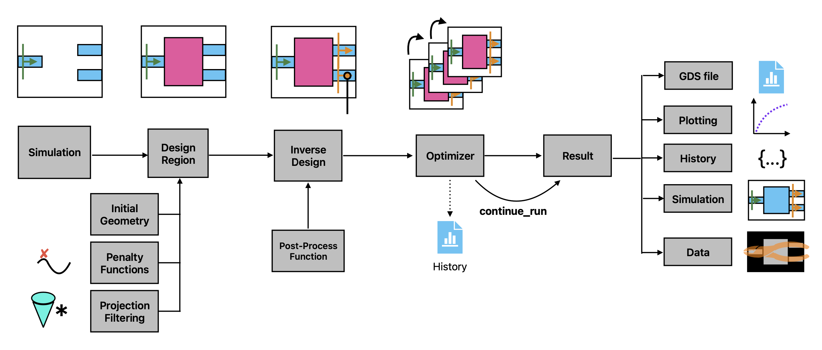
TidyGrad uses automatic differentiation (AD) to make this inverse designing process as simple as possible. The TidyGrad simulation code is integrated directly within common platforms for training machine learning models. TidyGrad informs these platforms how to compute derivatives for FDTD simulations using the adjoint method and the AD tools handle the rest. As a result, one can write an objective function in regular python code involving one or many Tidy3D simulations and arbitrary pre and post processing. Then gradients of this function are computed efficiently using the adjoint method, with just a single line of code and without deriving any derivatives.
The simulations are backed by cloud-based GPU solvers, making them fast and enabling large scale 3D inverse design problems.
Why is it better than the other similar tools?
Other products require their users to use one of a select few supported operations. This is extremely limiting when designing objectives that do more than just the very basic operations. Because TidyGrad leverages automatic differentiation to handle everything around the simulation, native python and numpy code are all differentiable, making possible extremely flexible and custom metrics. We can support differentiation with respect to most of our simulation specifications and data outputs, enabling tons of possibilities.
TidyGrad’s adjoint code is general, well tested, and backed by massively parallel GPU solvers making it extremely fast. And the front end code interfaces seamlessly with python packages for machine learning, scientific computing, and visualization.
How to use TidyGrad?
All the user needs to do is write their objective as a regular python function metric = f(params) taking the design parameters and returning the metric as a single number. Then a single line of code can transform this function into one that returns the gradient using the adjoint method gradient = grad(f)(params). The resulting gradient can be plugged into an open source or custom optimizer of your choice. See the example for for inspiration.
How to quickly get started?
No matter whether you are a GUI user or Python enthusiasts, we recommend you start from this document and then go through a couple of examples after thatf. If you want to focus on GUI, we have prepared an example for you.
If you want a refresher on the concepts first, the inverse design course by Tyler and Shanhui is a useful tutorial. Tyler’s presentation is a useful introduction from fundamental physics to practical applications.
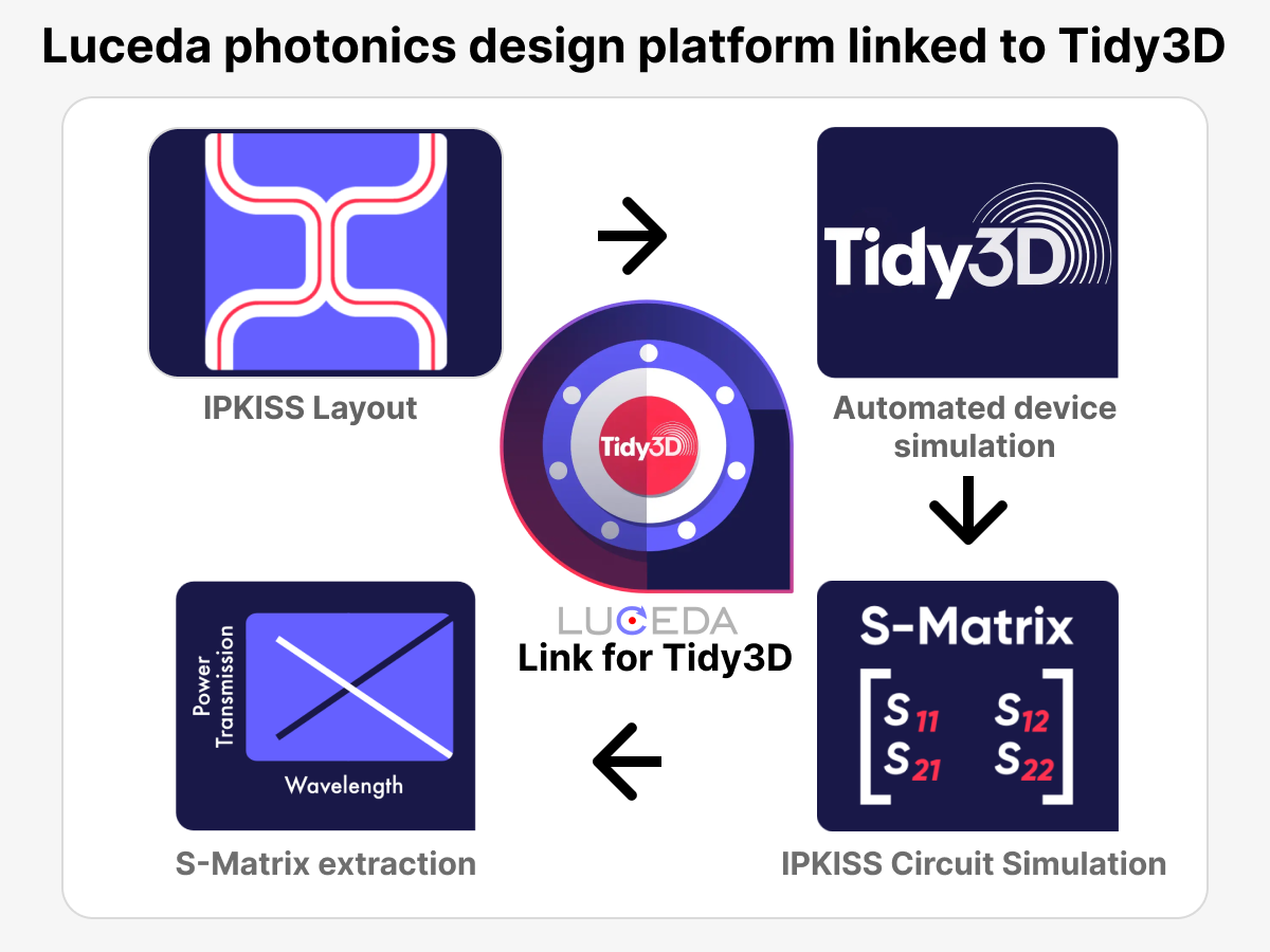
Luceda Photonics, a leading provider of photonic design automation solutions, announced a new integration with Tidy3D, a cutting-edge electromagnetic simulation solver from Flexcompute. This collaboration marks a significant advancement in photonic device design, offering users unprecedented efficiency and accuracy in their workflow.
The integration between Luceda Photonics’ powerful photonic integrated circuit (PIC) design platform and Tidy3D’s state-of-the-art FDTD simulation engine allows designers to streamline the process of creating, simulating, and optimizing photonic devices, from start to finish, on a single platform.

The key benefits of Luceda Photonics’ integration with Tidy3D include:
- Seamless Workflow: Users can now easily transfer designs from Luceda’s photonic integrated circuit (PIC) design platform to Tidy3D for fast and efficient electromagnetic simulations.
- Advanced Computational Power: Tidy3D’s high-performance computing capabilities, powered by hardware acceleration, ensure that even complex photonic devices are simulated with unparalleled speed and accuracy.
- Comprehensive Design Tools: The combined platforms provide a complete toolkit for photonics engineers, enabling them to perform both the design and simulation stages without switching between different software environments.
- Enhanced Collaboration: The integration supports collaboration between design teams, enabling them to efficiently iterate on PIC designs and simulations, leading to faster innovation and reduced time-to-market.
How it works:
The new integration allows the PIC designing on Luceda’s photonic platform and electromagnetic simulations running in Tidy3D. Users can visualize simulation results and adjust their designs with minimal hassle, ensuring a smooth and responsive design process. Additionally, users benefit from Tidy3D’s unique cloud-based hardware acceleration, making large simulations more accessible than ever.
Luceda Photonics and Flexcompute are committed to empowering engineers and researchers with the most advanced tools in photonics design. By bridging the gap between design and simulation, this partnership promises to transform how photonic devices are created and optimized across industries, including telecommunications, quantum computing, and sensing.
For more information on the Luceda Photonics and Tidy3D integration, visit https://www.lucedaphotonics.com/link-for-tidy3d.
FONEX Data Systems Inc., a leader in telecommunications innovation, is at the forefront of providing cutting-edge network infrastructure solutions across Canada and Europe. With their newly established R&D section, FONEX is pushing the boundaries of integrated external cavity lasers, a technology with far-reaching applications in telecommunications and various other areas.

FONEX ‘s R&D team found themselves facing a significant challenge when investigating the various integrated optical components, particularly micro ring resonators. The complexity of these interactions demanded powerful simulation tools that could provide accurate results without consuming excessive time and resources. Tidy3D has helped transform FONEX’s research and development process. The R&D team quickly realized that Tidy3D offered a unique combination of fast speed, high accuracy, and timely technical support that set it apart from other simulation tools in the market.
“Tidy3D has significantly improved our workflow with its exceptionally fast simulation processing times and reliable support team. It is an invaluable tool in our research and development of integrated lasers,” – Dr. Mohsen Rezaei, R&D engineer at FONEX.
The primary advantages of Tidy3D are its remarkable simulation speed and responsive support team. This allows FONEX to iterate designs rapidly, explore more parameters, and accelerate their innovation cycle while minimizing downtime. Moreover, Tidy3D is backed by a highly responsive support team, ensuring that any issues encountered during the simulation process are quickly addressed and resolved. This level of support has proven crucial in maintaining the momentum of FONEX’s research efforts, minimizing downtime, and maximizing productivity.
As FONEX continues to innovate, Tidy3D evolves alongside them, continuously enhancing its features and capabilities. This partnership exemplifies how advanced simulation tools can drive innovation in high-tech industries, helping translate visionary ideas into practical, patentable technologies.
As the telecommunications landscape continues to evolve, with increasing demands for faster, more efficient networks and more sensitive detection systems, the work being done at FONEX promises to play a crucial role. Their advancements in technology have the potential to unlock new possibilities in network infrastructure, paving the way for the next generation of telecommunications technology.
In the rapidly evolving field of proteomics, Pumpkinseed is making waves with its novel approach to protein sequencing. By leveraging advanced silicon photonic devices, this innovative biotechnology startup is working towards providing light-speed reads of the proteome, potentially revolutionizing our understanding of cellular processes and opening new avenues for therapeutic development. Pumpkinseed’s ambitious goal is to develop an optics-based approach to protein sequencing that can scale to the full complexity of the complete proteome. Unlike traditional methods that rely on complex biochemical probes, Pumpkinseed’s technology utilizes silicon photonic devices to sensitively extract the vibrational “fingerprint” of protein molecules without the need for any biochemical probes or labels.
|
|
|
|
Company LOGO (left) and a schematic illustration of Pumpkinseed’s advanced protein sequencing technology. |
|

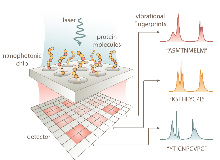
“Proteins are critical to a wide array of cellular processes - from cell signaling to immune responses, nutrient transport, growth, and metabolic regulation,” explains Dr. Jack Hu, co-founder of Pumpkinseed. “Our improved understanding of the presence and sequence of proteins could inform new disease pathways and lead to new therapeutics.”
At the heart of Pumpkinseed’s innovative approach lies the design and optimization of nanophotonic sensor chips. This is where Tidy3D plays a crucial role. The Pumpkinseed team utilizes Tidy3D to enhance their sensor designs, enabling more efficient extraction of optical signals from protein molecules of interest and allowing for the physical miniaturization of devices to pack millions of sensors onto a single chip.
“The primary advantage of Tidy3D is the incredible speed of the simulations,” Dr. Hu emphasizes. In the fast-paced environment of a biotechnology startup, where projects across multiple disciplines need to converge simultaneously, Tidy3D’s speed is invaluable. It allows the team to rapidly iterate on chip designs, improving device performance while saving time and costs on actual semiconductor manufacturing. Moreover, Tidy3D’s Python API has proven to be a game-changer for Pumpkinseed’s multidisciplinary team. It enables them to quickly design simulation experiments and analyze and visualize results. This has led to a significant speed up of communication of results and findings across the multi-disciplinary team and enabled improved R&D progress across the entire team.
The impact of Tidy3D on Pumpkinseed’s work extends beyond just simulation speed. By facilitating rapid design iterations and enabling efficient communication of results, Tidy3D has become an integral part of Pumpkinseed’s R&D process. It has allowed the team to bridge the gap between nanophotonic design, optical and fluidic instrumentation, and chemistry – all crucial elements in their innovative approach to protein sequencing. The partnership between Pumpkinseed and Tidy3D exemplifies how advanced simulation tools can drive innovation in biotechnology, potentially leading to breakthroughs that could transform our understanding of cellular processes and pave the way for new therapeutic approaches.
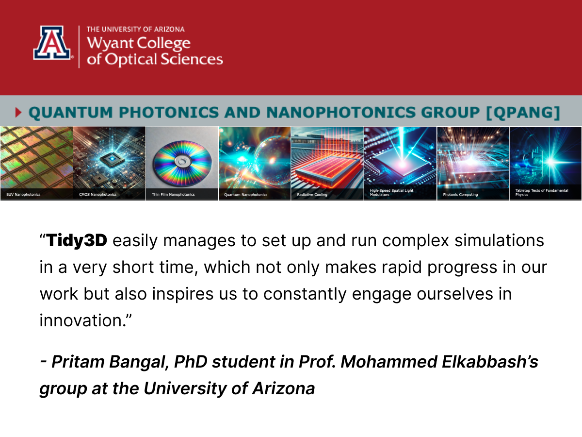
At the forefront of nanophotonic innovation, the Quantum Nano-photonics group at the University of Arizona is making significant strides in developing state-of-the-art technologies for the future. Led by Prof. Mohammed Elkabbash, Assistant Professor at the Wyant College of Optical Sciences, the group is tackling complex challenges in quantum optics, industrial photonics, and optoelectronics.

Prof Mohamed ElKabbash’s research lab at the University of Arizona
 
|
Professor Mohamed ElKabbash (left) and PhD student Pritam Bangal (right).
Pritam Bangal, a PhD student in the group, kindly shares insights into their groundbreaking work and how Tidy3D is accelerating their research efforts. “Our group aims to pioneer cutting-edge nanophotonic technologies with transformative applications in quantum optics, industrial photonics, and optoelectronics,” Pritam explains. Their ambitious goals include advancing quantum computing and communication through innovative photonic devices, enhancing industrial optical systems, and developing next-generation optoelectronic components.
The group’s research spans the entire spectrum of innovation, from design and simulation to fabrication and application. Their projects are as diverse as they are impactful. Pritam has been using Tidy3D for over a year, working on various research projects including guided mode resonance structures and designing optical nano-antennas to enhance the spontaneous emission rate from quantum emitters for potential use in quantum computing.
More recently, the group’s focus has shifted towards UV and Extreme UV Nanophotonics. Pritam is working on designing optical elements in the EUV (13.5nm) range for potential use in EUV lithography. He is successful in designing metalens with better efficiency in both visible and UV (50 nm) range. The impact of Tidy3D on the group’s work is significant. As Pritam notes, “Tidy3D easily manages to set-up and run complex simulations in a very short time which not only makes rapid progress in our work but also inspires us to constantly engage ourselves in innovation.”
The software’s efficiency and ease of use have accelerated the research cycle, allowing the team to focus more on analysis and innovation rather than troubleshooting. This has been particularly beneficial for new students in the group, encouraging them to learn and use FDTD tools in their research.
As the Quantum Nano-photonics group continues to push the boundaries of light manipulation at the nanoscale, Tidy3D remains a cornerstone of their research toolkit. The partnership between this innovative research group and Tidy3D exemplifies how advanced simulation tools can drive progress in cutting-edge scientific fields, potentially leading to technological breakthroughs that revolutionize industries and enhance our scientific understanding.
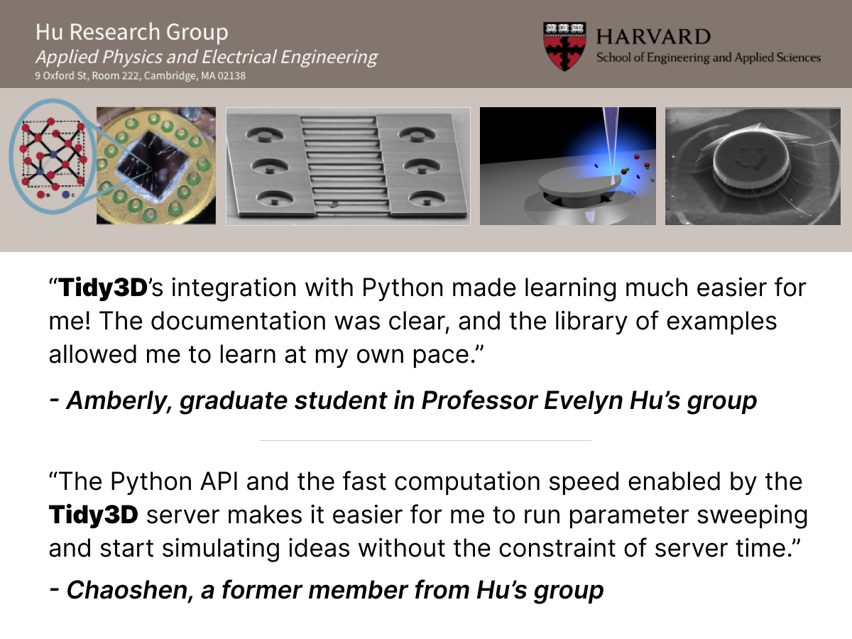
Professor Evelyn Hu’s research group from the School of Engineering and Applied Sciences at Harvard University is at the forefront of nanoscale optical and electronic research. The group is pushing the boundaries of light-matter interaction through innovative designs and nanofabrication techniques in 4H-silicon carbide and silicon. Their groundbreaking works in cavity-defect interactions and electrical control of defects have opened new avenues for probing fundamental material physics and developing high-performance devices for both classical and quantum applications.
, Silicon Carbide and Diamond (top right), GaN (bottom left), and Two-Dimensional Materials (bottom right)") |
| Prof Evelyn Hu’s researches on Silicon Color Centers (top left), Silicon Carbide and Diamond (top right), GaN (bottom left), and Two-Dimensional Materials (bottom right){: .align-center} |
 |
| Prof Evelyn Hu’s group at a dinner gathering |
The Hu group is an early adopter of Tidy3D. “Tidy3D’s integration with Python made learning much easier for me!” says Amberly, a graduate student in the group. “The documentation was clear, and the library of examples allowed me to learn at my own pace.” This accessibility has been particularly valuable for team members new to FDTD simulations, lowering the entry barrier to advanced nanophotonic design.
The group has leveraged Tidy3D for various projects, including the simulation of a novel photonic crystal cavity design in 4H-SiC. This new design promises more reliable and facile fabrication, potentially advancing the field of nanophotonics.
Chaoshen, another member of the research team, highlights the software’s versatility: “The Python API and the fast computation speed enabled by the Tidy3D server makes it easier for me to run parameter sweeping and start simulating ideas without the constraint of server time.” This capability has significantly enhanced the group’s ability to explore and optimize complex designs.
The batch sweep feature has proven particularly valuable in the optimization of photonic structures. Chang, a graduate student focusing on structure optimization, notes, “The batch sweep feature is very helpful in optimizing our photonic structures.”
Beyond the software’s technical capabilities, the Hu research group found the support from the Flexcompute team to be exceptional. “The team at Flexcompute was super helpful and very responsive to any questions I had,” Amberly shares. “I was even able to send them snippets of my code for them to look through, and they were fast at helping me debug and better understand what was going on.”
As the Hu research group continues to push the boundaries of nanoscale light-matter interaction, Tidy3D remains an invaluable tool in their research arsenal. The combination of computational power, user-friendly interface, and responsive support has enabled the team to accelerate their simulations, explore more complex designs, and ultimately, advance the field of nanophotonics. The group’s experience with Tidy3D exemplifies how advanced simulation tools can drive innovation in cutting-edge research, helping translate visionary ideas into groundbreaking discoveries.
Pixel Photonics is a pioneering deep-tech start-up founded in 2021 as a spin-off of the University of Münster and based in Münster, Germany. The company has developed a unique approach for integrating superconducting nanowire single-photon detectors (SNSPDs) on a chip waveguide. Pixel Photonics combines the superior features of SNSPDs with the versatility of an integrated photonic platform to deliver highly parallelized, efficient, and ultra-fast single-photon detection.
|
|
|
|
Photographs of the photonic chip (left) and SNSPD products (right) of Pixel Photonics |
|
")
")
While SNSPDs are inherently threshold detectors and insensitive to the number of photons in a detection event, waveguide integration and parallelization enable using SNSPDs for photon counting, thus paving the way for high-performance and scalable photonic quantum computing.
One of the biggest challenges of Pixel Photonics’ unique approach to SNSPDs is efficient fiber-to-chip coupling from an external source to our on-chip platform, the design of which requires large-scale nanophotonic computation.
“Tidy3D helps us to perform these computations in a matter of minutes,” says Dr. Marek Kozon, R&D Engineer for Computational Optics at Pixel Photonics.
Using Tidy3D, Dr. Kozon, and his team have designed couplers that exceed the previous generation’s efficiency while allowing for a smoother design process.
“I especially value the flexibility of Tidy3D, which is seamlessly integrated within the Python environment. This means that we are not dependent only on currently implemented software features but can extend the functionality ourselves to whatever suits our needs. I also like that all the data files are transparent, and there are no hidden or encoded files, which, again, makes it very smooth to work with Tidy3D.”
Photonic design engineers like Dr. Kozon are revolutionizing photonic industries. We at Flexcompute proudly provide efficient tools to their excellent hands. At the same time, we help guide our customers through their simulation journey by providing complementary and timely technical support. Dr. Kozon says, “I have been delighted with the approachability and knowledge of the customer service.”
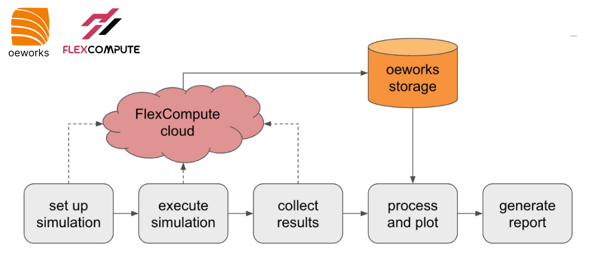
Who is oeworks
At oeworks we create solutions that empower technology innovators to rapidly advance their ideas from concept to prototype to production. We have worked on a large number of technical challenges across several domains and have developed and continue to evolve a toolkit consisting of hardware, software, and processes, including several commercial simulation tools. We structure our work using a technical risk mitigation framework, which, in conjunction with our toolkit, allows us to define and traverse the shortest path between a technical challenge and its solution.
Why we chose Tidy3D
When working on a design project, we typically use a combination of analytical models and simulations to better understand and mitigate technical risk. Once we achieve a fundamental understanding of the design landscape, we want to complete parametric explorations and quickly obtain precise results at specific design points.
Tidy3D has been a game change for us in a number of ways. The most obvious one is speed. Thanks to its substantial hardware acceleration, Tidy3D enables us to complete parametric simulations on a range and scale that were previously impractical, if at all possible.
A second advantage of Tidy3D is that it allows us to define our simulations as Python code. This enables us to streamline the process of defining simulations, particularly when we have the need to parametrize them. It also allows us to integrate many tools from the rich Python ecosystem, ranging from optimization and simulation orchestration to results storage, processing, and visualization. We have been able to generate code that, using a single command, can set up a number of parametric simulations, execute them, collect and store the results, and then process, interpret, and plot them. In some instances where the reporting requirements were known a priori we have even been able to generate the complete reports in slide format.
 |
| Figure 1: Process flow from simulation set up to report generation. The entire process can be executed using a single command. |
Another advantage of simulation-as-code is that it can easily be integrated into our revision control system. Given the large number of projects we execute and the often rapidly evolving parameter spaces we are required to explore, this gives us a great advantage in tracking the evolution of our simulations and designs. Furthermore, it enables reproducibility in the event that we need to revisit a result or resume work that has been paused for a substantial period of time.
|
|
|
|
Figure 2: Far field emission patterns of micro-LED structures for different polarizations. |
|


We also had a great experience with Tidy3D from an IT infrastructure point of view. Simulation setup is very lightweight and can be worked on any of the standard development machines we routinely use. Simulation execution runs on Flexcompute’s cloud instances, freeing us from the requirement to acquire, operate, and maintain high-end workstations. In addition to that, license setup is practically trivial, freeing precious IT resources for an operation of our size.
|
(a) |
(b) |
|
Figure 3: Post-processing of light extraction simulation results. (a) Far-field radiosity vs. elevation angle; (b) Light extraction efficiency vs. a design parameter for two different configurations. |
|
 Far-field radiosity vs. elevation angle")
 Light extraction efficiency vs. a design parameter for two different configurations")
Finally, we have been delighted with the support we have received from the Flexcompute team. All our requests for support have been addressed promptly, and without fail we were pointed in the right direction, minimizing downtime. We have also interacted with the development team and have found them to be very responsive to our requests for enhancements and new features.
Conclusion
Since we adopted Tidy3D as our main FDTD simulation tool, we have used it to complete many projects, ranging from micro-LED light extraction optimization to the modeling of silicon photonic components. Our clients have been very satisfied with our ability to quickly explore extended design spaces and simulate large structures with quick turnaround times. Internally, we have been able to streamline our workflows for simulation setup, execution, and result processing and visualization, leading to drastically improved efficiency.
Our engagement with the Flexcompute support and development teams has been extremely smooth and productive – we have the highest confidence in their ability to support us in our efforts to accelerate our client’s technology release to market.
We are continuously improving our understanding of Tidy3D’s evolving capabilities and are actively seeking projects that can benefit from streamlined FDTD simulations in the context of a thorough understanding of the corresponding design space. We look forward to discussing how our processes and software tools, combined with the power of Tidy3D, can help mitigate your technical risk, and allow you to reach your objectives faster.

We at Flexcompute are thrilled to have collaborated with NVIDIA to push the boundaries of scientific computing! Together, we have explored the incredible potential of 𝗚𝗣𝗨-𝗮𝗰𝗰𝗲𝗹𝗲𝗿𝗮𝘁𝗲𝗱 𝗽𝗵𝗼𝘁𝗼𝗻𝗶𝗰 𝗦𝗶𝗺𝘂𝗹𝗮𝘁𝗶𝗼𝗻𝘀, leveraging the latest hardware advancements to solve Maxwell’s equations at unprecedented speed and scale.
Our collaboration showcases how NVIDIA’s cutting-edge GPUs power AI and revolutionizes how we approach complex physical simulations. The possibilities are endless, from reducing simulation times by orders of magnitude to enabling the design and optimization of next-generation photonic devices!
𝗪𝗵𝘆 𝘁𝗵𝗶𝘀 𝗺𝗮𝘁𝘁𝗲𝗿𝘀:
𝗦𝗽𝗲𝗲𝗱: simulations that once took hours can now be completed in minutes
𝗦𝗰𝗮𝗹𝗲: we can simulate larger and more complex devices, accelerating innovation in photonics
𝗔𝗰𝗰𝘂𝗿𝗮𝗰𝘆: advanced simulations allow for more precise designs, pushing the limits of what’s possible
See the publication here.
This collaboration is just the beginning. As we continue to explore and develop these technologies, we are excited about the future of scientific computing and the breakthroughs that lie ahead.
Thanks to the amazing teams at Flexcompute and NVIDIA for making this possible. Here’s to driving innovation forward!

Renowned for its expertise in diamond photonics, the Lončar Lab at Harvard University has expanded its focus to lithium niobate in recent years, pioneering new avenues in the fabrication of photonic structures. The Lončar Lab has developed sophisticated in-house fabrication technologies, which can be used to quickly test the performance of designed devices. However, designing lithium niobate photonics often requires the designers to explore a large parameter space, which means too many chips must be fabricated and tested. Therefore, it’s critical to have a reliable numerical simulation tool to help with the design. Unfortunately, traditional 3D full-wave simulations are very slow. Tony Song, currently a graduate student from the Lončar Lab, and his teammates often rely on their efficient fabrication techniques and excellent testing capabilities for the parameter tuning of their designs rather than running numerical simulations. As another workaround, Tony also used to run highly simplified simulations to model devices, which is often not sufficiently accurate.
Recently, Tony and his teammates discovered Tidy3D. With the help of Tidy3D’s ultrafast simulations, they have already had exciting results that will be published in top scientific journals. Currently, Tony and his colleagues mainly use Tidy3D to design diamond photonic crystal cavities and passive lithium niobate components such as directional and grating couplers. In addition, they have also started to use inverse design to optimize some passive components.
Tony highly praised the well-designed user interface of Tidy3D compared to other simulation tools he has tried previously. The intuitive Python API of Tidy3D integrates effortlessly into his existing workflow, and the capabilities for importing and exporting GDS files facilitate a smooth transition between simulation and actual cleanroom fabrication. Moreover, Tony has commended the technical support team at Tidy3D for their prompt and effective assistance. Tony ran a broadband simulation in one specific case, but the result obtained had a strange discontinuity in the lower end of the wavelength range. Puzzled by the result, Tony contacted Tom and Emerson, the Senior Photonics Engineers at Flexcompute. They did a test together to identify the issue. “They helped me think a different way about the problem. Looking back, you might feel the solution was rather obvious, but it would have taken me a long time to figure that out myself. It’s always helpful to reach out to [Flexcompute’s] experts and get their opinion on the matter,” said Tony.
However, Tony and his teammates’ long-term goal is to explore active components utilizing the large electro-optic coefficient and nonlinear coefficients of lithium niobate. This vision aligns perfectly with Tidy3D’s development blueprint as the Tidy3D team continues to develop more advanced nonlinearity features and multi-physics solvers. These additions enable more rigorous simulations in thermo-optic and electro-optic domains, which is essential for the work Tony and his lab aspire to undertake.
The success story of Tidy3D in the Lončar Lab underscores the software’s pivotal role in advancing nanophotonics research. From its user-friendly interface and fast simulation speed to its advanced features, such as nonlinearity and inverse design plugins, Tidy3D has proven to be a transformative tool. As the Lončar Lab continues to explore new frontiers in photonics, Tidy3D stands as an essential companion, empowering researchers to unlock novel insights and accelerate the pace of discovery in the ever-evolving field of nanophotonics.


Flexcompute is proud to share that the National Academy of Engineering (NAE) has elected our co-founder Dr. Shanhui Fan to its 2024 Class for showing that “the coldness of space” relative to Earth can be a major energy source for humankind.

Dr. Shanhui Fan also serves as Joseph and Hon Mai Goodman Professor of the School of Engineering, Electrical Engineering at Stanford University in Stanford, California. His induction into the NAE comes on the heels of Shanhui Fan’s previous accolade, where he was awarded Optica’s R. W. Wood Prize in 2022.
He is also the second member from Flexcompute to join the ranks of the NAE, following in the footsteps of Dr. Philippe Spalart. Flexcompute is honored to support excellence and leadership in engineering.
With this news, Flexcompute’s highly-recognized team continues to make waves in the simulation technology space with its award-winning research and by developing cutting-edge electrodynamics and Computational Fluid Dynamics (CFD) solvers.

The Finite-Difference Time-Domain (FDTD) method is a computational modeling technique widely used in the field of photonics. FDTD has significantly changed the way researchers study and predict the behavior of electromagnetic waves. This review article delves into the recent applications of FDTD simulations in cutting-edge photonics research and engineering. Specifically, it showcases examples of the use of FDTD simulations in areas such as novel 2D materials (such as graphene and transition-metal dichalcogenides), quantum technologies (like quantum dots and single photon light extraction), and consumer-grade electronics (such as CMOS image sensors).
2D materials in photonics
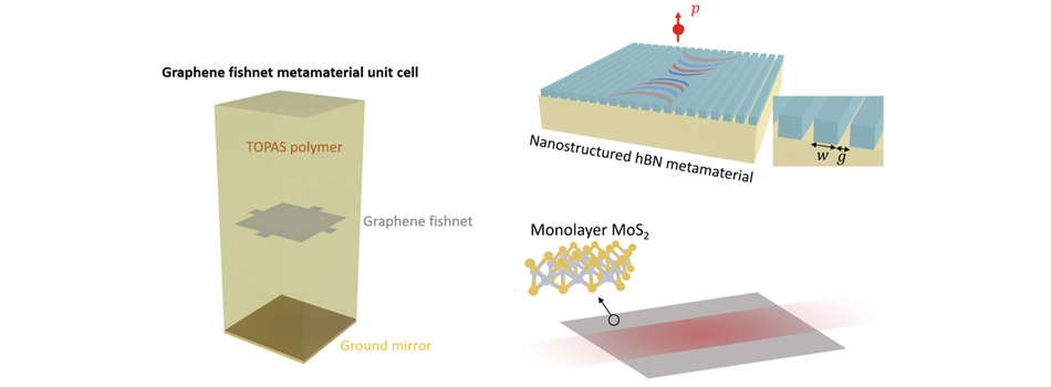
The emergence of 2D materials represents a significant breakthrough. These ultra-thin materials, often mere atoms in thickness, demonstrate unique electronic, optical, and mechanical properties, markedly different from their bulk forms. Graphene, a monolayer of carbon atoms in a honeycomb lattice, exemplifies this with its exceptional conductivity and transparency. Beyond graphene, 2D materials like TMDs, black phosphorus, and hexagonal boron nitride (hBN) have been identified, each with distinctive optical properties. These materials have facilitated novel applications in photonics, including ultrafast photodetectors, flexible optoelectronics, advanced photovoltaic cells, and light-emitting diodes (LEDs). The nanoscale manipulation of light using these 2D materials paves the way for innovative developments in communication technologies, energy harvesting, and quantum computing, marking a transformative phase in photonics.
Our example library showcases various photonic devices that are integrated with 2D materials. Some examples include the graphene metamaterial absorber, the nanostructured hBN with hyperbolic polaritons, and the waveguide made of MoS2 monolayer.
Photonic components for next-gen quantum technology
The rapid advancement of quantum technology is significantly influenced by the development of sophisticated photonic components, essential for driving the next generation of quantum systems. These components, encompassing single-photon sources, detectors, and integrated photonic circuits, form the foundation of quantum communication, computing, and sensing. They enable precise photon manipulation and control, facilitating critical quantum phenomena such as entanglement and superposition. In quantum computing, photonic elements are instrumental in generating and manipulating qubits, the quantum bits that exist in multiple states simultaneously, thereby significantly enhancing computing capabilities. In quantum communication, these components are crucial for establishing highly secure channels through quantum key distribution (QKD). Furthermore, progress in integrated quantum photonics is leading to more compact and robust quantum devices, advancing their practical application in various sectors, including secure data transmission and high-precision measurements. As ongoing research pushes the limits of current technology, photonic components are poised to be key in harnessing the full potential of quantum technology, ushering in a new era of information processing and other applications.
Our example library features several quantum photonics-related examples, including the Bullseye cavity quantum emitter light extractor, the inverse-designed quantum emitter light extractor, and the Plasmonic Yagi-Uda nanoantenna.

Photonic devices in consumer-grade electronics
The integration of advanced photonic devices in consumer electronics is markedly enhancing user experiences, as seen in the use of CMOS image sensors in digital imaging as well as Fresnel lenses and diffractive gratings in augmented reality (AR) and virtual reality (VR) systems. CMOS sensors, notable for their low power consumption and high-quality imaging, are crucial in smartphones and digital cameras, capturing high-resolution images with excellent clarity and color fidelity. These sensors utilize photonics to convert light into electronic signals, resulting in the vivid, detailed digital images prevalent in modern devices. In AR and VR, Fresnel lenses, known for their concentric ring structure, offer a lightweight, thin alternative to traditional lenses, ideal for compact headsets. They effectively bend light for immersive visual experiences while reducing headset bulk, enhancing user comfort during prolonged use. CMOS image sensors and Fresnel lenses demonstrate the significant role of photonic technologies in consumer electronics, driving innovation and expanding the possibilities of user interaction in digital environments.

Conclusion
The advancements in technology have led to a significant increase in the demand for faster and more efficient computing methods. Photonic devices are becoming increasingly important in modern technology, and the demand for faster and more accurate electromagnetic simulations is growing. FDTD has been a critical tool in advancing the development of photonic devices, but conventional FDTD solvers can no longer keep up with the speed of technological development. Novel hardware-accelerated FDTD tools like Tidy3D are designed to overcome the limitations of traditional FDTD solvers. These tools leverage the power of modern computing hardware to deliver faster and more accurate simulations, making it possible to design and optimize photonic devices at a scale and speed that was previously impossible. With the advent of these innovative tools, a new era of photonic device development is emerging, one that promises to deliver faster, more efficient, and more reliable technology.
The field of integrated photonic circuits has seen a significant and rapid expansion in recent years, with strong indications of continued acceleration in the near future. This growth is largely fueled by innovative academic research.
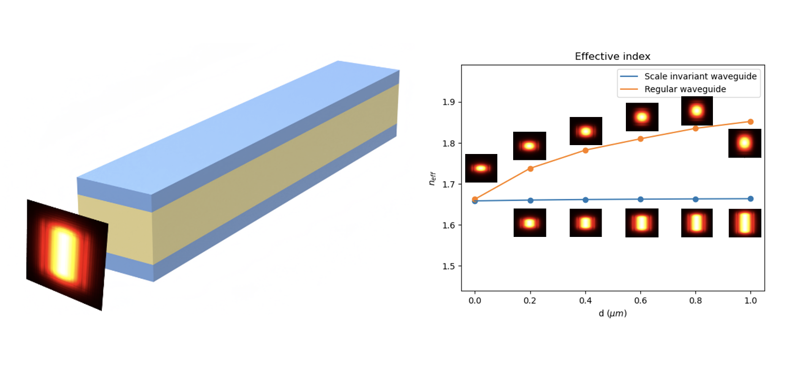
A notable example of such advancement is the study led by Dr. Janderson Rodrigues and Dr. Utsav Dave from Professor Michal Lipson’s team at Columbia University, as detailed in a recent publication in Nature Communications. This research introduces a new dielectric waveguiding mechanism. Their novel waveguide design effectively traps light within materials of low refractive index on a chip. The study reveals that at a specific threshold, the transverse wavevector transitions from imaginary to real, consequently forming an optical mode that remains consistent and scale-independent, regardless of the geometry. This phenomenon results in significant light localization within a low-index layer, presenting a substantial advancement in the field.

The waveguide design presented in the study is highly intriguing. We replicated the simulations described in the original paper, presenting them as a public example. Our simulation results align closely with both the theoretical predictions and the experimental observations reported in the study.
We had the privilege of interviewing Dr. Janderson Rodrigues and Dr. Utsav Dave, who graciously offered insights into their research. We are immensely grateful for the time and effort they devoted to this discussion. The following is the complete interview transcript, encompassing the questions and their insightful responses.
1. What inspired the initial concept for the scale-invariant waveguide design in the paper?
We were working on an unrelated project in which the goal was to reduce the evanescent fields in order to avoid the coupling between parallel waveguides. By analyzing the corresponding equations, it turns out that it is easier to increase the evanescent field instead of decreasing it. At the limit, the field becomes flat before it becomes radiation modes. This inflection point is exactly the cut-off condition of the asymmetric waveguide and therefore is an unstable point (the critical angle). We realized that two parallel waveguides operating at this condition would lead to a flat mode. Later we found out that something similar has been predicted in plasmonic waveguides, which helped us to understand the effect with the huge advantage of using only (lossless) dielectric materials.
2. What advantage does the scale-invariant waveguide have over conventional dielectric waveguide?
Janderson: One of the main advantages of the scale-invariant waveguide is the increasing overlap of the field intensity with low-index materials, mainly in heterogeneous structures, due to the limited number of alternative approaches. For this purpose, beyond the critical point is even more attractive. Furthermore, a flat mode distribution means a uniform distribution of light throughout the middle material (large mode effective area), which can be interesting to avoid non-linear effects or tailor the saturation of gain medium, for instance. Besides that, the starting point of increasing the evanescent coupling (i.e., shorter directional couplers) still can be explored.
Utsav: Besides, since the scale invariant waveguide has the same effective index as the low-index material width is changed, devices with different dimensions can retain the same overall phase shift, which can be useful in optimizing different structures without worrying about realigning phase shifts.
3. How do the uniform field distribution and non-Gaussian spatial profile in your waveguides impact their potential applications in integrated photonics? How do you envision the application of scale-invariant waveguides in the future?
Although, the paper shows the experimental demonstration in the telecommunication range, the same concept can be applied to other regions of the electromagnetic spectrum, for example, the visible or the terahertz range. We also notice that the proposed structure might find applications in electro-optic modulation, nonlinear integrated photonics, and temperature control.
4. What are you working on currently?
Janderson: Currently, I am working in the private sector in the field of integrated photonics and trying to find a good balance between my interest in basic science with the necessity of product development and engineering.
Utsav: I am working in a proteomics company where we use integrated photonics for single-molecule sensing of proteins, helping to usher in the next revolution beyond genomics.
5. Can you give some suggestions to students who want to work in the field of photonics?
Janderson: If I can give any suggestions for students in the field, it would be to use toy models. The fact that we can play with these relatively simple equations of 1D slab waveguides before going to more rigorous numerical simulations, was one of the greatest pieces of advice that was given to me.
Utsav: Photonics is both a great applications-oriented platform as well as a playground for exploring all kinds of cool physics like nonlinear dynamics, non-Hermitian or topological physics, etc. So you may not know from the beginning what kind of work/topic you like and the best way to know is to try a bunch of things. Try and get a broad overview of all aspects - from theory to fabrication and experiment. This will help you whether you end up in industry or academia (or something else). It’s also important to make sure that the research group culture where you will be spending your master’s or PhD matches your personality and is nurturing - that by far is the most important factor to success.
Author Bios
 Janderson Rocha Rodrigues was born in Sao Paulo, Brazil, in 1980. He received the Microelectronics Engineering Diploma from the Sao Paulo State Technological College (FATECSP), Sao Paulo, Brazil, in 2008 and the M.S. and Ph.D. degrees in Space Science & Technologies Engineering from the Aeronautics Institute of Technology (ITA), Sao Jose dos Campos, SP, Brazil in 2011 and 2019. From 2018 to 2019, he was a Ph.D. visiting student at Michal Lipson’s group at Columbia University, NY, USA, where he rejoined as a postdoctoral Research Scientist from 2019 to 2023. Since 2023, he has been a Research Scientist at Corning Inc., NY, USA. His research interests include applications of integrated photonics to communications as well as to sensing and instrumentation.

Utsav D. Dave, originally from western India, completed his B. Tech. nestled in the foothills of the Himalayas in 2010 from the Indian Institute of Technology, Guwahati. He then went on to do a M.S. in Photonics jointly from a group of UK and European universities through the Erasmus Mundus program followed by a PhD in integrated silicon photonics from Ghent University, Belgium. He later moved to Michal Lipson’s group at Columbia University as a postdoc in 2017 where he worked on subwavelength and non-Hermitian photonics, LiDAR and frequency combs before joining Quantum-Si in 2022 where he currently works on photonics for proteomics using single-molecular spectroscopy.

Prof. Michal Lipson is the Eugene Higgins Professor at Columbia University. Her research focus is on Nanophotonics and includes the investigation of novel phenomena, as well as the development of novel devices and applications. She is the inventor of over 45 issued patents and has co-authored more than 250 scientific publications. In recognition of her work in silicon photonics, she was elected as a member of the National Academy of Sciences and the American Academy of Arts and Sciences. Her numerous awards include the NAS Comstock Prize in Physics, the MacArthur Fellowship, the Blavatnik Award, Optica’s R. W. Wood Prize, the John Tyndall Award, the IEEE Photonics Award, and an honorary degree from Trinity College, University of Dublin. In 2020 she was elected the 2021 Vice President of Optica, formerly known as The Optical Society, and will serve as Optica President in 2023. Since 2014, every year she has been named by Thomson Reuters as a top 1% highly cited researcher in the field of Physics.

As we gather to celebrate this festive season, we at Flexcompute want to extend our heartfelt holiday greetings to you and your loved ones. This time of year reminds us of the warmth of community, the joy of innovation, and the bright future we’re building together.
🌟 This year, we’re grateful for the brilliant ideas and collaborative efforts that have propelled us forward. Like the steady glow of a holiday candle, our commitment to advancing CFD and EM simulations continues to burn bright.
🎅 Merry Christmas and a Happy New Year! 🎇
Here’s to a season of joy, a new year of breakthroughs, and a future filled with incredible possibilities.
Flexcompute hold a seminar at Harvard on Dec 14. In the seminar, Dr Tom Chen presented Hardware-accelerated Photonic Inverse Design.
Inverse Design is a technique that uses computational methods to automate the process of designing photonic devices. It plays an important role in photonic design for academic research and industrial engineering.
Tom’s lecture was highly praised by the audience. After the presentation, Tom and Marjon had a deep discussion with the students about their simulations and help them troubleshooting the problems.
Don’t worry if you was not able to attend the semianr. Access the presentation slides here!


Thank you for attending the Aero Tech Talks seminar featuring Dr. Jim Coder from Penn State. We hope you found his presentation and Q&A session on transition models insightful!
Did you miss the live event? You can catch up now by accessing the webinar recording here.
Stay tuned for our next Aero Tech Talks seminar in early 2024 - sign up to receive the latest news.


Thank you for attending our insightful webinar on Nov 30th: “The Future of Photonic Simulation and Device Design”! We trust you gained valuable insights from Dr. Momchil Minkov’s presentation and the engaging Q&A session.
Missed the live event? Catch up now by accessing the webinar recording here.
Stay informed about upcoming webinars and workshops — sign up to receive the latest news!

As the leaves turn and we gather to give thanks, all of us at Flexcompute want to extend our warmest Thanksgiving wishes to you and your loved ones. This day is all about gratitude, family, and the joy of togetherness, values we cherish deeply. We are extremely thankful for the incredible community that supports us.
We are also reminded of how computational physics, from fluid dynamics to electromagnetic simulations, brings us together in the spirit of innovation. Let’s continue to collaborate, innovate, and push the boundaries of what’s possible.
Wishing you a holiday filled with joy, innovation, and gratitude. 🌟

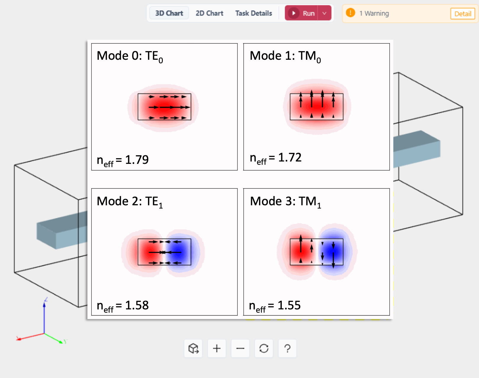
Working Principles
A mode solver is a computational tool used to find the electromagnetic field distribution – or mode profile – and the propagation constant (β) of modes in a waveguide, optical fiber, or other types of guiding structures. To understand how a mode solver works, we consider a simple case and start with Maxwell’s equations, assuming a time-harmonic field and isotropic nonmagnetic medium

where E is the electric field, H is the magnetic field, ω is the angular frequency, and ε is the permittivity. From Faraday’s Law, we have
![]()
which is equivalent to the system of equations

Similarly, from Ampere’s Law, we can obtain three additional equations

Here, each field component has a spatial dependence, e.g. Ex=Ex(x,y,z). Now without loss of generality we assume our mode solving plane is the xy plane and the guided mode propagates in the z direction. That is, we assume the fields have a z dependence of e-jβz. Combining this assumption with the system of equations above, we arrive at the new system of equations only for the transverse fields Ex(x,y), Ey(x,y), … as

This system of equations can now be numerically solved via different methods such as the finite difference method as implemented in Tidy3D’s mode solver. This calculation takes several steps:
1. Discretization of the Computational Domain
First, the cross-section of the waveguide is divided into a grid where each point on the grid will have an associated electric and magnetic field value. The grid can be uniform or non-uniform. The grid size needs to be sufficiently fine to resolve the mode profile.
2. Finite Difference Approximation of Derivatives
The partial derivatives in the equations are replaced with finite differences. For example, the derivative of Ex with respect to y at point i,j can be approximated as

where Δy is the spacing between the grid points in the y direction.
3. Forming the Algebraic System
Once the partial derivatives are replaced with finite differences, the equations turn into algebraic equations. The discretized equations for every point in the domain form a large matrix equation
![]()
where A is a matrix representing the coefficients from the finite difference approximations of the equations. X is the vector of unknowns (field components at each grid point).
4. Solving the Algebraic System
Solving this large system of equations becomes an eigenvalue problem that can be solved numerically. Each eigenvalue corresponds to a different mode’s propagation constant, and each eigenvector gives the corresponding mode’s field distribution.
Applications
1. Waveguide and Optical Fiber Design and Analysis
There are several occasions where we would like to run the mode solver. First of all, the mode solver is essential for waveguide design. Photonic researchers and engineers can use it to calculate mode profiles, effective indices, group indices, and polarization properties. See the following tutorials to learn how to use mode solver as well as the waveguide plugin in Tidy3D:
Tutorial 1: Using the mode solver for optical mode analysis
Tutorial 2: Using the waveguide plugin to analyze waveguide modes
2. Mode Coupling and Conversion Analysis
Furthermore, mode solver is an important tool in coupler and splitter designs. When designing a coupler or splitter, we often need to compute the phase matching condition, which requires accurate calculation of the effective indices of different modes on different waveguides. Based on the mode solving results, one can also derive other quantities of interest such as the overlap integral of two modes, which indicates mode matching and efficiency in mode conversion. We demonstrate mode analysis for coupler design in the following examples:
Example 1: Polarization splitter and rotator based on 90 degree bends
Example 2: 8-Channel mode and polarization de-multiplexer
Example 3: Broadband directional coupler
Example 4: Exceptional coupling for waveguide crosstalk reduction
Example 5: Broadband bi-level taper polarization rotator-splitter
3. Excitation Mode Inspection
In FDTD simulations for photonic components, we often use a mode source to introduce a specific mode into the simulation as excitation, while using mode monitors to track mode transmission and conversion. Before running the FDTD, we can use the mode solver to inspect all the supported modes at the input waveguide and ensure that the desired one is selected as the source, as demonstrated in the following examples:
Example 1: Waveguide Y junction
Example 2: Photonic crystal waveguide polarization filter
Example 3: Plasmonic waveguide sensor for carbon dioxide detection
Notice that both the mode source and mode monitor utilize the same mode-solving algorithm under the hood, and they are used ubiquitously in integrated photonics related examples such as
Example 1: Inverse taper edge coupler
Example 2: Uniform grating coupler
Example 3: Focusing apodized grating coupler
Example 4: Thin film lithium niobate adiabatic waveguide coupler
Example 5: 1x4 MMI power splitter
Example 6: Compact polarization splitter-rotator
Example 7: THz integrated demultiplexer/filter based on a ring resonator
When exploring computational electromagnetic (EM) tools, you’ll find many commercial and open-source options. Among these, Tidy3D stands out for several reasons. Tidy3D is an electromagnetic simulation tool based on the finite-difference time-domain (FDTD) method, and it’s built on a modern computing architecture. This allows for scalable, accurate simulations at speeds unmatched by other products in the market. The unique benefits of Tidy3D make it a compelling choice over other simulation tools for those looking for enhanced performance and reliability in electromagnetic simulations. In this blog article, we discuss five key advantages of Tidy3D.
Finish Your Simulations in a Coffee Break
In the past, running full-wave simulations, such as a metalens in the visible frequency range, would often require engineers to wait extended periods of time. Sometimes, simulations would take days or even weeks to complete, forcing engineers to run them overnight or on weekends. However, Tidy3D takes advantage of advanced parallel computing chips, which significantly speeds up the simulation process. This acceleration allows simulations that used to take an entire day to be completed in just a short coffee break. You can refer to our speed benchmark for a detailed understanding of the improved simulation speeds that Tidy3D provides. Experience the ultra-fast simulation from the examples Adjoint-based shape optimization of a waveguide bend, 1x4 MMI power splitter and Metalens in the visible frequency range.
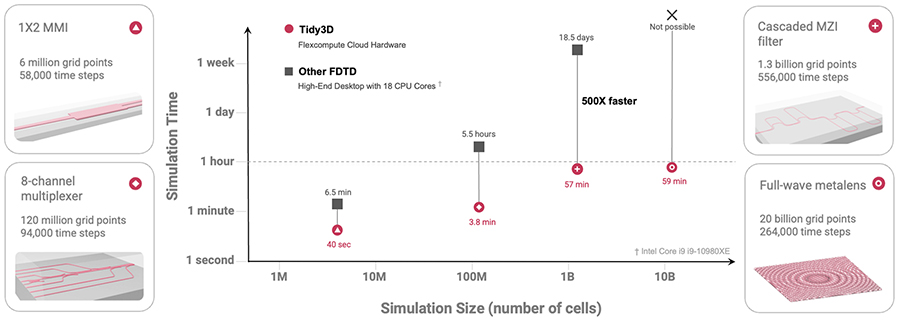
Scalability to Thousands of Wavelengths in Size
Conventional EM solvers face a major challenge in terms of scalability. While solving EM problems on a small scale is manageable, real-world device simulations require the analysis of structures that span hundreds or thousands of wavelengths. Such large-scale simulations, for example, the 3D optical Luneburg lens, require significant hardware resources that may not be accessible to many engineers and researchers.
To address this challenge, Tidy3D has implemented a cloud-based computation paradigm. By utilizing an intelligent algorithm, computational hardware resources are dynamically allocated for each simulation task submitted by users. This ensures that there are adequate hardware resources available for every simulation, optimizing the performance. Tidy3D has successfully conducted FDTD simulations with up to 50 billion grid points for our clients, which was previously unimaginable.
Rigorous Full-wave Simulation Without Approximation
Various EM solvers employ approximation methods to enhance efficiency in solving certain problems. A notable example is the beam propagation method, which hinges on the slowly varying envelope approximation. While such approximation methods expedite large simulations, they often compromise accuracy, leaving results open to question.
In contrast, the FDTD method employed by Tidy3D is a full-wave method. This means it rigorously solves Maxwell’s equations without resorting to any approximations. Utilizing Tidy3D for modeling your device eliminates guesswork, thereby instilling full confidence in your design outcomes. See the example of a Full-wave simulation of a millimeter-scale waveguide coupler below.
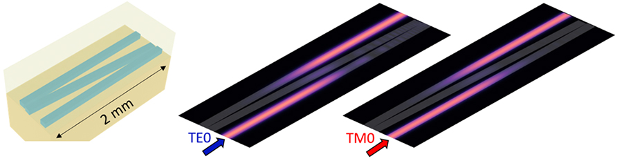
Flexible Python and GUI interfaces
Traditional simulation software often provides either a scripting API or a graphical user interface with limited scripting capabilities. However, Tidy3D offers the best of both worlds. Our adaptable Python API facilitates the programmatic definition of complex simulations, allowing for seamless integration with other open-source Python libraries. This, in turn, empowers you to achieve intricate functionalities with Tidy3D and customize it to fit your existing photonic design workflow.
At the same time, we provide a web-based graphical user interface that offers a visually intuitive experience. This interface allows for swift inspection of your simulation setup and results, delivering both visual and operational advantages.
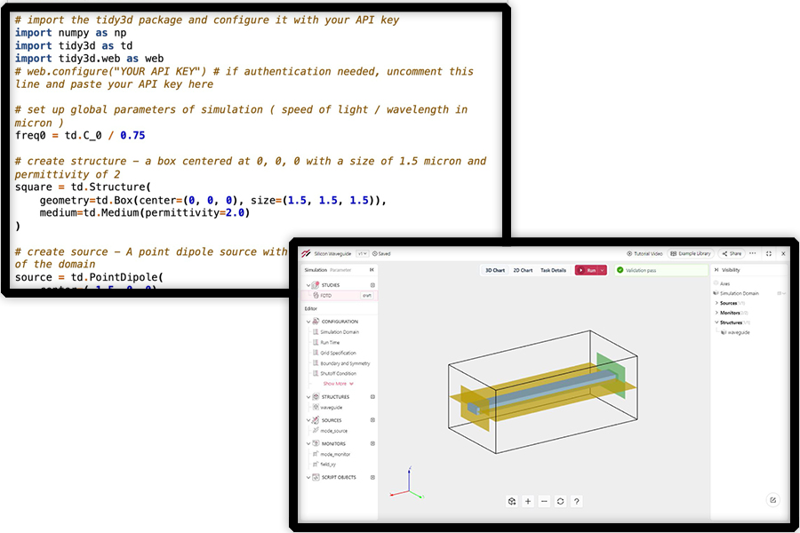
Timely Technical Support at Your Fingertips
Our Tidy3D users come from various backgrounds and experience levels. No matter your expertise, we understand that you might have some questions about how to use Tidy3D. As a Tidy3D user, you will have access to our technical support team, made up of experienced engineers and leading researchers in the relevant field.
Our objective is to provide a resolution to your technical support request within one business day in most cases. Our solver is ultrafast, and we aim to complement it with equally swift technical support to provide a first-class user experience that is unmatched by other commercial products.
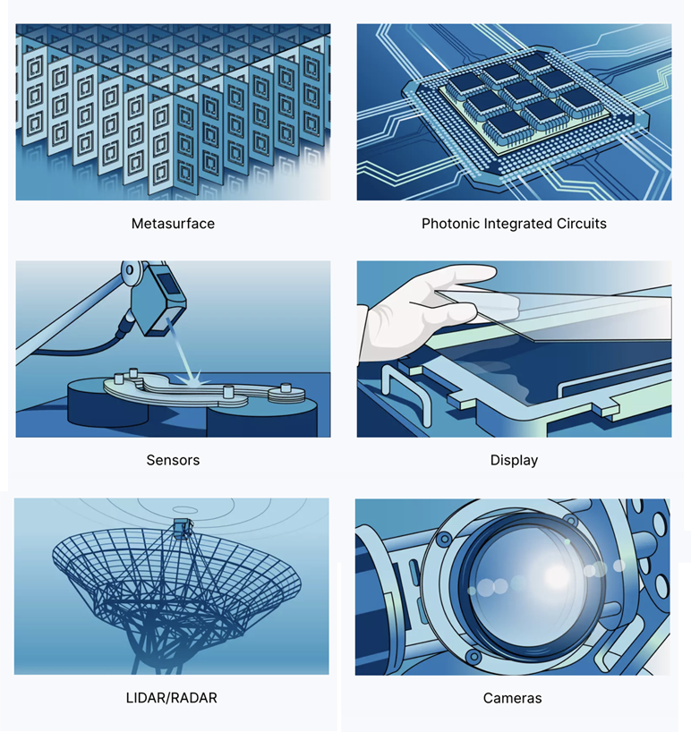
The finite-difference time-domain (FDTD) method, as implemented in Tidy3D, is used to rigorously solve Maxwell’s equations to quantitatively describe the complex interactions of electromagnetic waves with different materials and structures. It has found a plethora of applications spamming a wide frequency range, from below radio frequency (RF) in the MHz scale to above ultraviolet (UV) with a wavelength below 100 nm. FDTD simulations are widely used in device design, validation, and verification across many fields, including telecommunications, integrated photonics, lens design, metamaterials, photonic crystals, plasmonics, and so on. In this article, we explore some of the key categories where FDTD is an indispensable tool.
Photonic Integrated Circuit Component
Photonic integrated circuits (PICs) are at the forefront of optical technology, merging multiple photonic functions onto a single chip. Similar to how electronic integrated circuits revolutionized electronics by miniaturizing and combining numerous electronic components, PICs are doing the same with optical elements. They use light to transmit and process information, which allows for higher speeds, greater data bandwidth, and less energy consumption compared to traditional electronic circuits. In addition, PIC can be designed to work as lidar or sensitive environmental sensors. Recent research and development also point to PIC as a promising platform for future quantum computers.
Complex PICs contain various functional components, such as waveguides, couplers, splitters, modulators, resonators, etc. FDTD is the most widely used tool for designing and optimizing integrated photonic components. In the realm of integrated photonic component modeling, the primary focus is on the propagation of waveguide modes. The ModeSource and ModeMonitor combination in Tidy3D can be used to launch and detect specific waveguide or fiber modes. The ModeSolver plugin is capable of computing various mode properties, such as effective index, group index, and mode profile. The ComponentModeler plugin can be used to calculate the scattering matrix elements of a multi-port device. Last but not least, the adjoint plugin enables Tidy3D users to design high-performance components with a compact footprint through inverse design. See more examples of various PIC components below.
- Waveguide
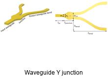
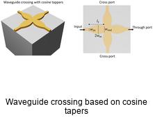
- Waveguide coupler, convertor, grating and resonator
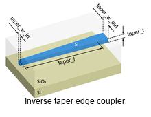
 .
. 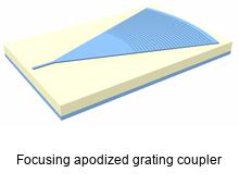
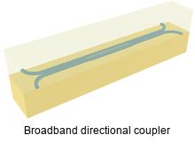
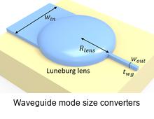 .
. 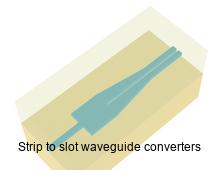
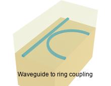
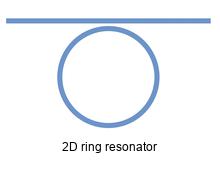
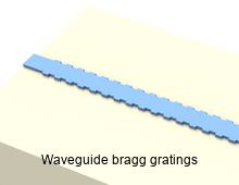
- Splitter
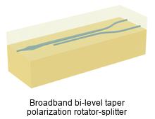
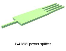 .
. 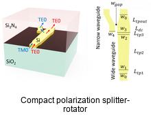
- De-mutiplexer and filter
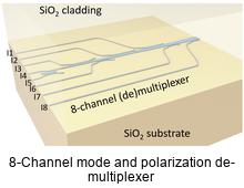
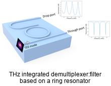
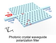
Periodic Photonic Structures
Periodic optical structures are a class of materials engineered to manipulate light in precise and often novel ways. This category encompasses a range of technologies, including metamaterials, metasurfaces, diffractive gratings, and photonic crystals, each with its unique approach to interacting with electromagnetic waves. Metamaterials are artificial materials with properties not found in nature, designed to bend and shape light in unconventional manners. Metasurfaces are the two-dimensional counterparts that allow for the control of light with subwavelength-patterned interfaces. Diffractive gratings split and diffract light into several beams, capitalizing on the wave nature of light to create interference patterns. Photonic crystals, structured with periodic dielectric or metal-dielectric materials, create a band gap for photons, influencing the propagation of light in much the same way that the periodic potential in a semiconductor crystal affects electrons.
With the convenient periodic boundary condition and Bloch boundary condition features, modeling periodic structures in Tidy3D is extremely easy and fast. On the other hand, we often need to model finite periodic structures since real-world devices always have a finite size. This kind of simulation is usually computationally intensive and that’s where the scalability and ultrafast speed of Tidy3D really shine.
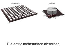
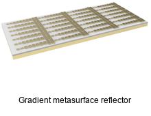
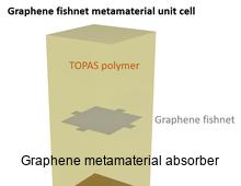
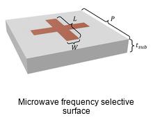
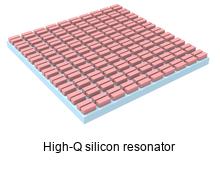
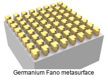
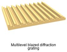
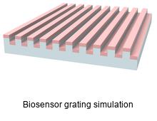
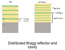
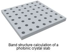
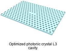
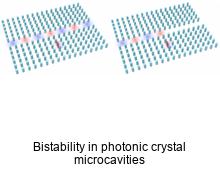
Optical Scattering and Far-field Radiation
Optical scattering and far-field radiation are fundamental concepts in the study of light behavior, crucial for understanding and designing a wide range of optical systems. Optical scattering refers to the deflection of light rays when they encounter irregularities or particles within a medium, causing light to spread in various directions. Far-field radiation, on the other hand, pertains to the region where light waves propagate freely after emanating from a source or after interacting with an object, typically considered when the distance from the source or object is significantly greater than the wavelength of the light. In this regime, the light waves can be approximated as plane waves, simplifying the analysis of optical systems.
Tidy3D offers several useful features that aid users in simulating optical scattering and far-field radiation. One of these features is the total-field scattered-field (TFSF) source, which acts as an artificial boundary within the simulation. It introduces the incident field into the total field region and ensures that only the scattered field is present in the scattered field region. By doing so, it makes it easier to calculate various scattering properties.
Additionally, the near-field to far-field projection monitors allow users to simulate a small domain and compute the fields far away based on the fields in the near-field region. For example, this feature is particularly useful for simulating large lenses with a long focal length.
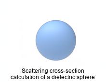
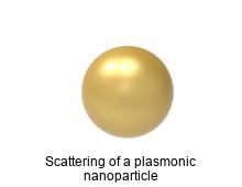
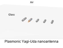
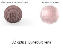
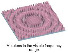
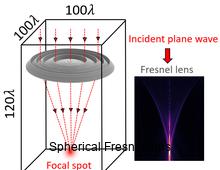
Other Nanophotonic Systems
Besides what’s been introduced previously, FDTD is also widely used in the modeling of various other state-of-the-art nanophotonic systems. Just to list a few:
- Plasmonics explores the interaction between electromagnetic field and free electrons in a metal. The ability of plasmonic materials to confine light into tiny volumes beyond the diffraction limit of light makes them extremely useful for a variety of applications, such as nanoantenna, sensors, etc..
- Polaritonics is a field that studies the behavior of polaritons, hybrid quasiparticles that blend the properties of light and matter, arising from the coupling of photons with excitations such as phonons or excitons in a solid.
- Topological photonics is a rapidly growing research area that applies the concepts of topological order, originating from condensed matter physics, to the manipulation of light.
- Photonics with 2D materials, such as graphene, MoS2, etc., represents a burgeoning research domain that leverages the unique optical properties of atomically thin materials, like graphene, transition metal dichalcogenides (TMDCs), and black phosphorus, to manipulate light at the nanoscale. See the example of Hyperbolic polaritons in nanostructured hBN.
The progress of these innovative fields requires tools that can solve Maxwell’s equations accurately, quickly, and at scale. Therefore, tools like Tidy3D will always remain at the forefront of engineering and academic research to power future technological breakthroughs.
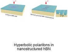
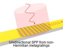
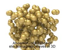
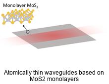
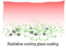
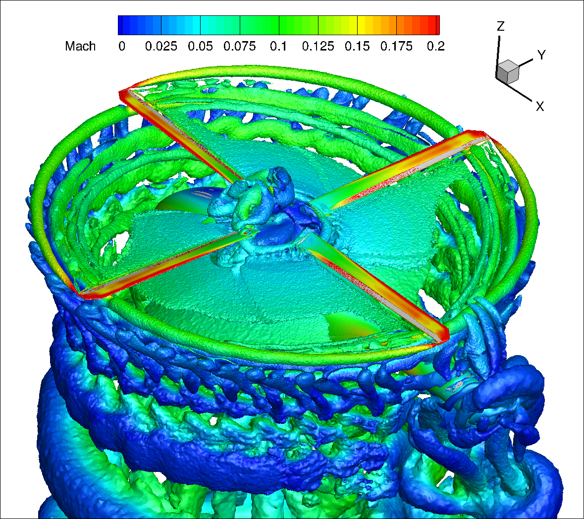
In this series of articles, we highlight our efforts to accurately model the flow physics of a hovering helicopter rotor in isolation and installed on a fuselage using the solver Flow360. In Part I, the motivation for the simulations was discussed. Part II provided details on the computational setup, including the rotor blade geometry, the Flow360 CFD solver, the treatment of turbulence, the computational grid, and the sliding interface methodology. Part III presents the simulation results, including the effect of mesh refinement and time resolution, collective sweep studies, and comparisons with experimental data and other CFD codes.
In this 3rd and last part of the series, we present the results we obtained by simulating a hovering rotor using our solver Flow360.
Definitions
Before presenting the results, let us first define the integrated loads and sectional loads. The thrust coefficient, torque coefficient and figure of merit (FoM) are defined as follows:
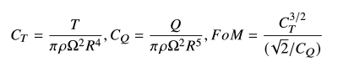
The sectional loads are normalized by the local chord and the local velocity as follows:
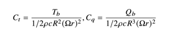
Isolated Rotor Setup
The integrated loads convergence for the isolated rotor with a mesh refinement and time step is shown in Figure 1. The FoM calculated from the integrated loads is plotted versus grid factor for different time steps, where N is the number of mesh nodes for the mesh refinement study. The power -⅔ for N would give straight lines with ideal 2nd-order convergence and in a family of grids.
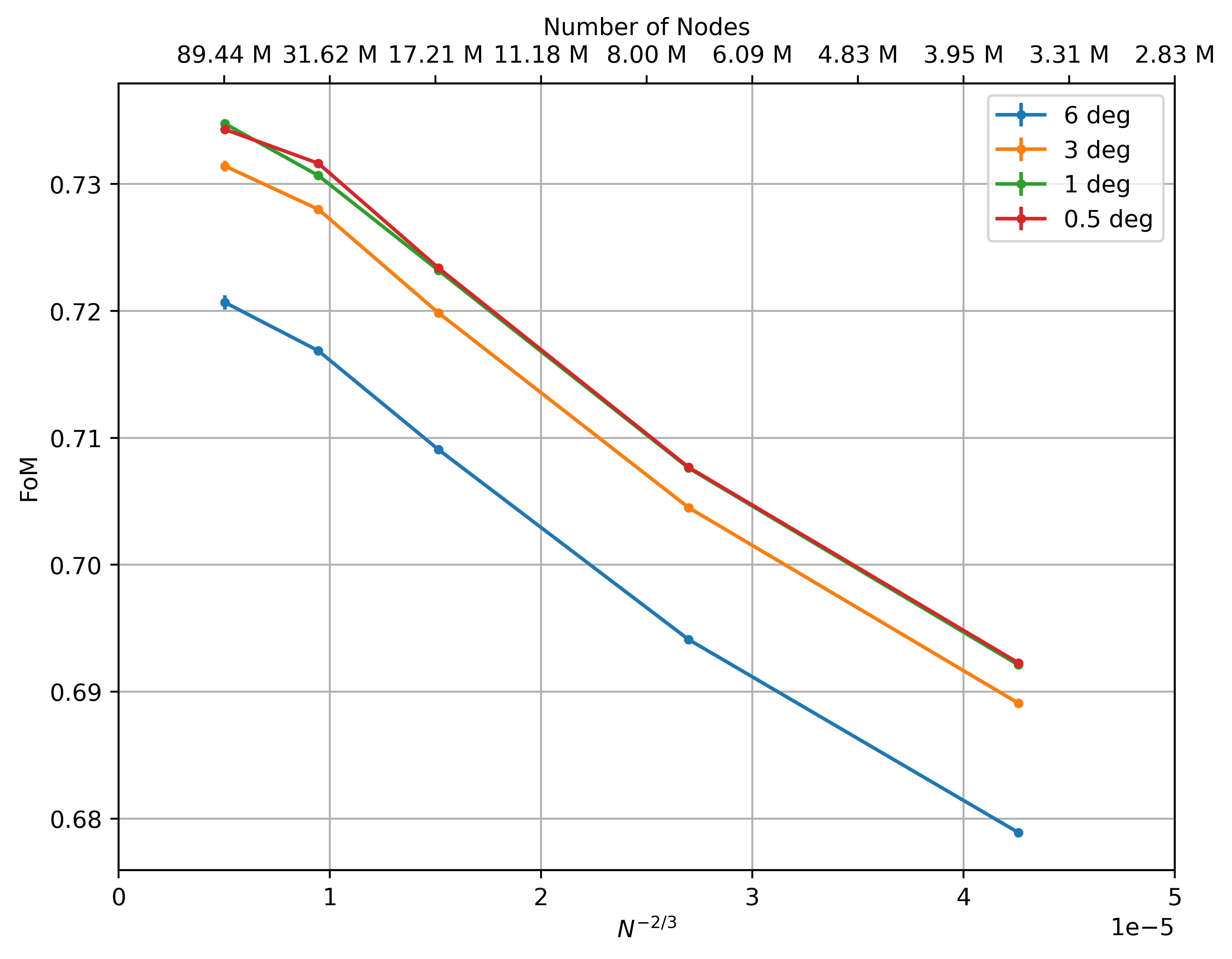
The first aspect worth highlighting is the close to negligible error bars for the integrated loads for the isolated rotor computations (not shown). A mesh refinement study shows that as the mesh is refined, the thrust and torque converge (not shown here). The increase in the FoM values as the time step is refined is primarily due to decreased torque values at finer time steps with minor differences for the finest two time steps.
The results are examined in further detail to explain the behavior of the integrated loads with mesh refinement and reduction in time step.

The sectional loads show a strong sensitivity to mesh refinement (Figure 2). Refinement of the mesh leads to a significantly better resolved tip vortex that has a large impact on the sectional loading inboard and outboard of approximately r/R = 0.9. Inboard, the preceding tip vortex induces downwash leading to a reduction in the local sectional loading, whereas outboard the tip vortex induces upwash leading to an increase in the local sectional loading. With mesh refinement, the location at which the tip vortex starts to impact the local loading also moves further inboard. Mesh refinement also leads to a reduction in local torque along the entire blade, especially in the location of the tip vortex. This is an example of favorable Blade-Vortex Interaction.
Let us now visualize the wakes using the Q-criterion colored with Mach number, shown in Figure 3. The wake visualizations show a strong dependency of the mesh on the resolved flow features away from the blade, whereas the dependency on the blade surface is weak except at the very tip. For the coarsest mesh, the tip vortices are poorly resolved. They are smeared at first, and later “end” because the Q criterion drops below the threshold level chosen. The solution highly resembles a blade-element theory solution where only a wide vortex tube is visible. As the mesh is refined the vortices are better resolved. The highest quality 5%c mesh shows instabilities in the rotor wake, which are seen in high-fidelity solutions in the literature. The secondary structures are due to the interaction of the tip vortices with the shear layers; thin shear layers are not marked by the Q criterion, by design. These structures are partly generated by the grid, which is not cylindrical, but braids are a well-known physical feature of mixing layers between the principal vortices.

Installed Rotor Setup
Let us now present the results for the installed rotor configuration which contains a fuselage. The integrated loads convergence for this setup with mesh refinement and time step reduction is shown in Figure 4. Note the much larger error bars on the integrated load predictions compared to the isolated rotor case (Figure 1). The primary reason for this is the presence of non 4/rev components with long transients in the loads, meaning that more rotor revolutions are required to obtain tighter error bars as well as the low number of samples used in the error bar computation. The rotor FoM value increases strongly with mesh refinement, but the time-step effect is weaker. All values of FoM fall within 0.5-a-count for time steps below 3 degrees and refinement level below 10%c, showing high confidence in the fine mesh/fine time step results.
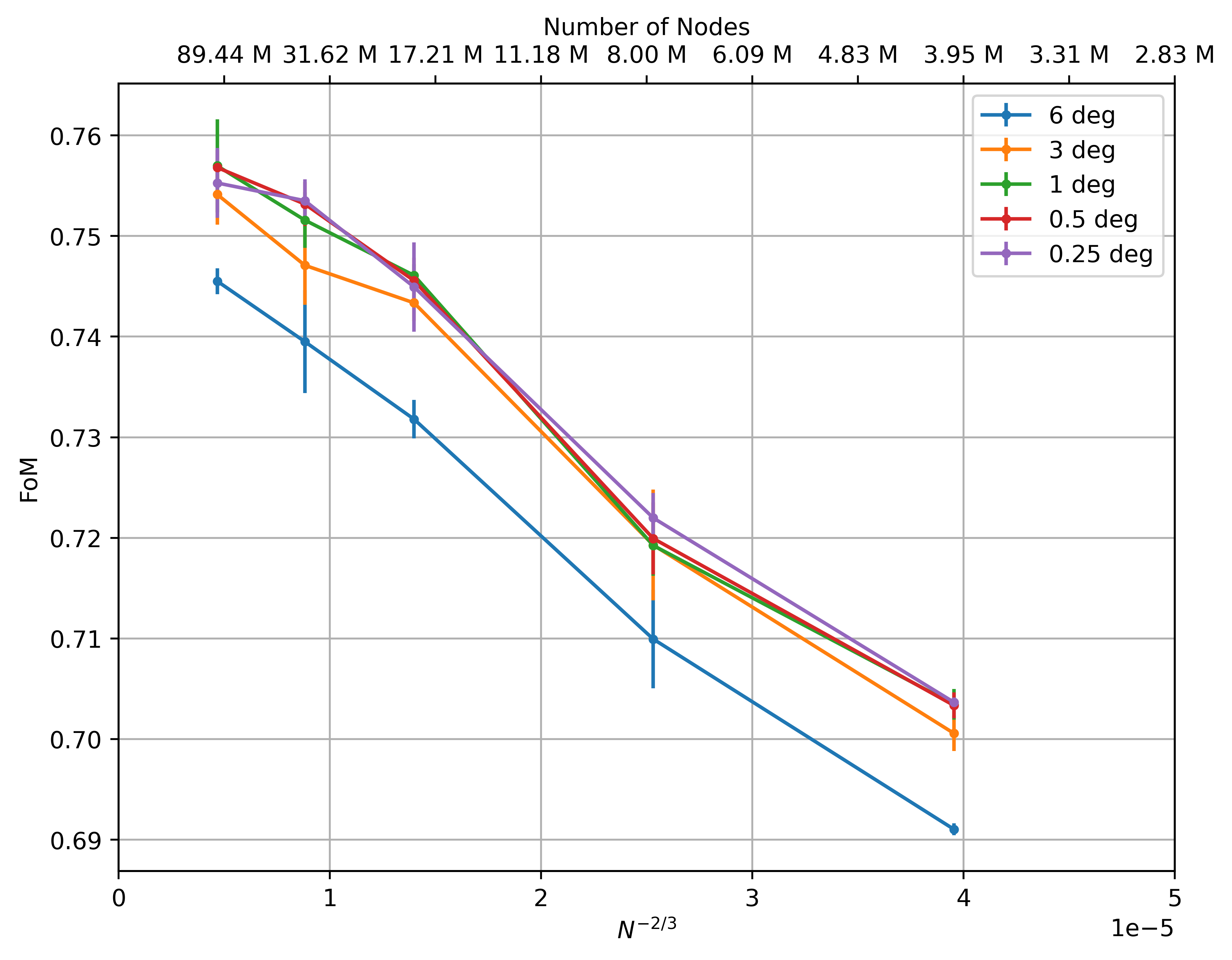
We also observed that the temporal convergence of the loads is much tighter for the isolated rotor than for the installed rotor. For instance, the FoM variation over 3 revolutions is less than 0.2 counts in FoM for the isolated rotor, while it is 0.5 counts in FoM for the installed rotor. This is because the isolated rotor does not have to interact with the fuselage, while the installed rotor does; see Figure 5. The “fountain” near the rotor axis is very noticeable, but is not very accurate when the hub itself is omitted. On the other hand, the distribution on the blade is quite close to that on the isolated rotor, although the pressure difference is clearly higher on the blade that is over the tail of the fuselage. The temporal oscillations in the loads for the installed rotor calculations are caused by vortex shedding from the fuselage. To reduce these errors, at least 20 revolutions should be simulated to obtain highly accurate integrated loads data.

Collective sweep study
We now present results from the collective sweep study. For the isolated rotor, we use the 5%c mesh with time steps of 0.5 degree, but for the installed rotor the time step is reduced to 0.25 degree. The study is performed at two blade tip Mach numbers, namely 0.58 and 0.65, and the results are compared to other CFD codes and experimental data in Figure 6.

The isolated rotor results show good agreement with experimental data and other CFD codes. Due to the nature of installed rotor calculations, however, this level of accuracy is deemed acceptable with values from longer averaging cycles to be obtained in the future.
Conclusions
In summary, we presented a rigorous mesh sensitivity and time step study for isolated and installed hovering rotor solutions, aiming to assess the level of discretization error sensitivity. Based on the results, a collective sweep was performed with the results compared to available experimental data and other CFD codes. We can conclude the following key points from our study:
- For isolated rotor solutions, 30-40 million nodes and a 1-degree time step are sufficient for engineering-level accuracy. There is evidence of second-order grid convergence.
- Finer time steps are needed for installed rotor simulations, and higher resolution solutions improve wake resolution but do not significantly improve performance predictions.
- Convergence for installed rotor simulations is more difficult due to slow transients and unsteady vortex shedding, resulting in higher uncertainties in load predictions.
- Unsteady DES-based simulations are necessary for accurate hover performance predictions, especially at high blade loading.
- Flow360 hover performance predictions are within 1 count of experimental data and 1-2 counts of other CFD codes.
- Fuselage download predictions are within 2% of reference data, with further investigation planned on statistical convergence requirements.
This concludes the series of articles we prepared on our simulation study of a hovering rotor. Stay tuned for more content from our CFD research efforts using Flow360!
If you’d like to learn more about CFD simulations, how to optimize them, or how to reduce your simulation time from weeks or days to hours or minutes, stop by our website at flexcompute.com or follow us on LinkedIn.
For the expanded version of the paper this content is derived from, click here.

In this series of articles, we highlight our efforts to accurately model the flow physics of a hovering helicopter rotor in isolation and installed on a fuselage using the solver Flow360. In Part I, the motivation for the simulations is discussed. Part II provides details on the computational setup, including the rotor blade geometry, the Flow360 CFD solver, the treatment of turbulence, the computational grid, and the sliding interface methodology. Part III presents the simulation results, including the effect of mesh refinement and time resolution, collective sweep studies, and comparisons with experimental data and other CFD codes.
In this 2nd part of the series, we present important details about the geometry of the rotor blades, the simulation grid, and the computational methods we used to model the hovering helicopter rotor.
Flow360 CFD Solver
Our simulation software, Flow360, is based on hardware/software co-design with emerging hardware computing leading to unprecedented solver speed without sacrificing accuracy. The Flow360 solver is a node-centered unstructured grid solver based on a 2nd order finite volume method. The convective fluxes are discretized using the Roe Riemann solver, whereas central differences are used for the viscous fluxes. MUSCL extrapolation is used to achieve higher order accuracy in space. Flow360 includes a number of standard turbulence models including SA-neg, SA-RC, 𝑘 − 𝜔 SST, and DDES. Transition modeling capabilities are also available based on the 3-equation SA-AFT model, but are not used in the present work. All simulations are performed as time-accurate using the dual time-stepping technique with the time derivative discretized using an implicit second-order accurate backward Euler scheme.
Geometry of the HVAB rotor blade
We focus on the 4-bladed HVAB rotor, which is the main topic of the Hover Prediction Workshop. We used the IGS file available on the hover prediction workshop file share site as the baseline blade geometry. As shown in Figure 1, the blade geometry is highly similar to the PSP rotor blade and features a planform with 14 degrees linear twist, RC-series airfoils and a swept-tapered tip (30 degrees sweep, 0.6 taper ratio outboard of 0.95 radius). The radius of the blade is 66.5 inches with a reference chord of 5.45 inches giving a rotor solidity of 0.1033. The flap hinge is located at 3.5 inches from the rotor axis with the lag hinge assumed to be coincident.
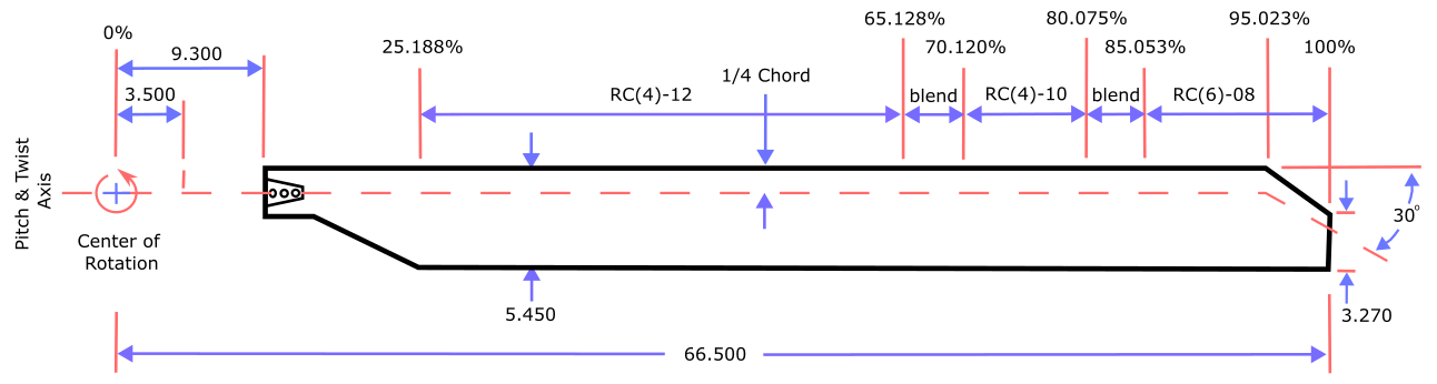
Fuselage
For installed rotor calculations, the NASA Robin-mod7 fuselage is used as recommended by the hover focus problem. This generic fuselage has an analytical definition with the cross sections defined by a series of superellipses. The fuselage geometry was generated in Engineering Sketch Pad (ESP) using 45 cross sections and compared visually to the Plot3D geometry available on the hover prediction workshop file share site. The geometry does not include the main rotor pylon or the rotor hub. The fuselage has a length of 123.931 inches and was pitched up by 3.5 degrees. The full configuration of the HVAB blades with the fuselage is shown in Figure 2.
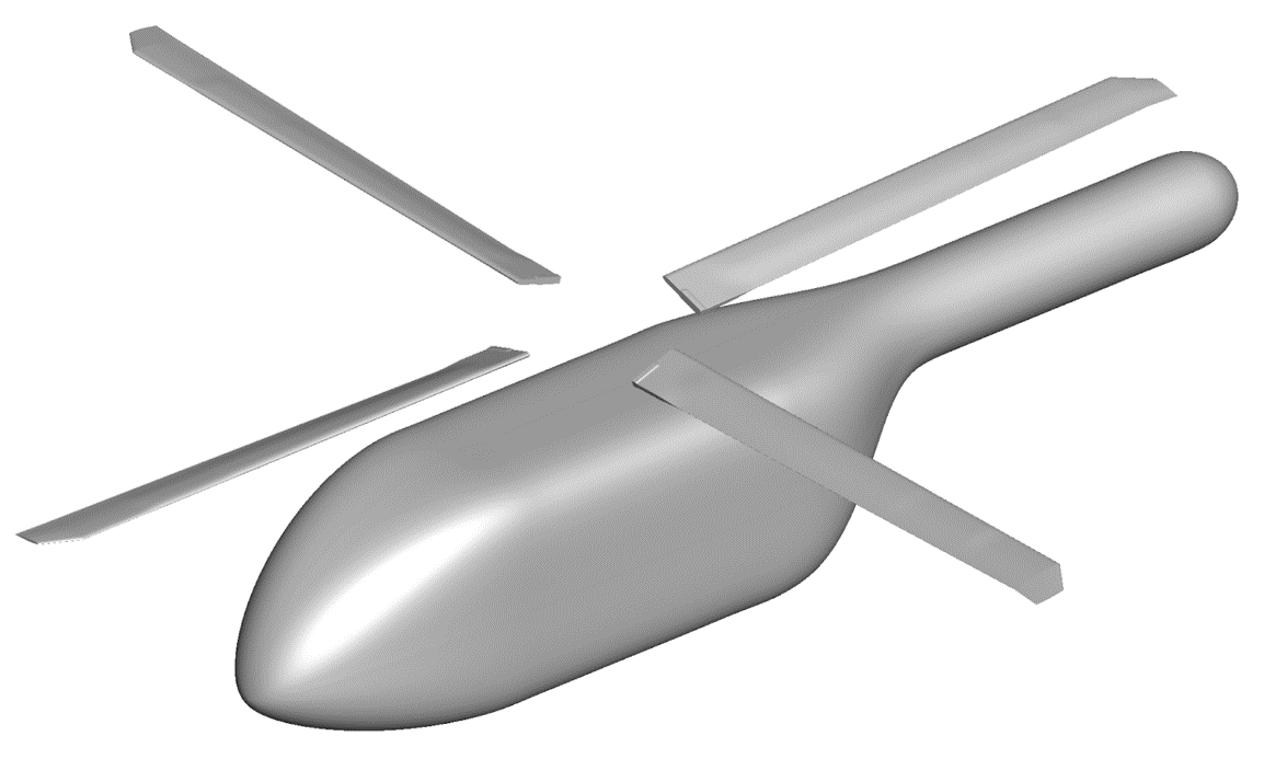
Sliding Interface Methodology
In order to efficiently simulate rotating blades, Flow360 solver uses the sliding interface methodology to model the relative motion of individual components. The domain is split into a nearfield rotating block which encloses the rotor blades and a farfield stationary block which contains the fuselage in the case of installed rotor cases. The blocks do not overlap. Data is interpolated between the two blocks in the y-z plane using a 2nd order scheme. To minimize the computational costs, strict constraints are imposed on the node layout on the sliding interface, as all nodes must lie on concentric circles, as shown in Figure 3. This leads to a significant reduction in computational overhead as no interpolation weights need to be calculated or stored as the position of each node is known at every time step.
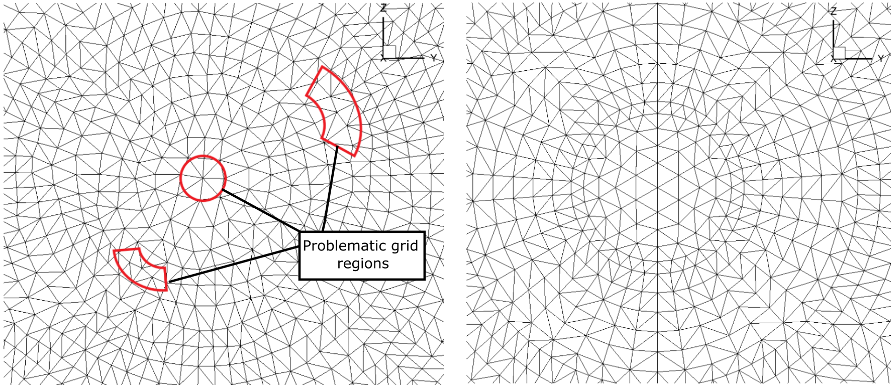
As the rotor was modeled using a sliding interface method for rotation, the meshes had to be regenerated for each collective angle and mesh refinement level. This was done by imposing the pitch, flap, and lag angles on the geometry through a series of translations and rotations.
To study the effect of mesh resolution, five mesh levels were generated and their resolution expressed in terms of the reference chord length (cref) of 5.45 inches. The values used were 20% cref, 15% cref, 10% cref, 7.5% cref (see Fig. 4), and 5% cref. For the surface mesh, the maximum edge length was set to 0.545 for the 10% cref mesh, and the refinement factor value was used to generate the other meshes. The curvature resolution parameter was set to 5 degrees to control the resolution at the leading edge, trailing edge, and blade tip.
The volume mesh used for this analysis is split into a rotating nearfield block and a farfield stationary block. The sliding interface is placed between -0.075R and 0.105R to allow anisotropic layers to grow on the fuselage surface. Wall-normal spacing is set to ensure 𝑦+<1 on the surfaces. The mesh uses hexahedral elements in the blade boundary layers and prism elements in the fuselage boundary layer, which transition to a tetrahedral mesh in the farfield. Three levels of refinement are used to resolve the wake.
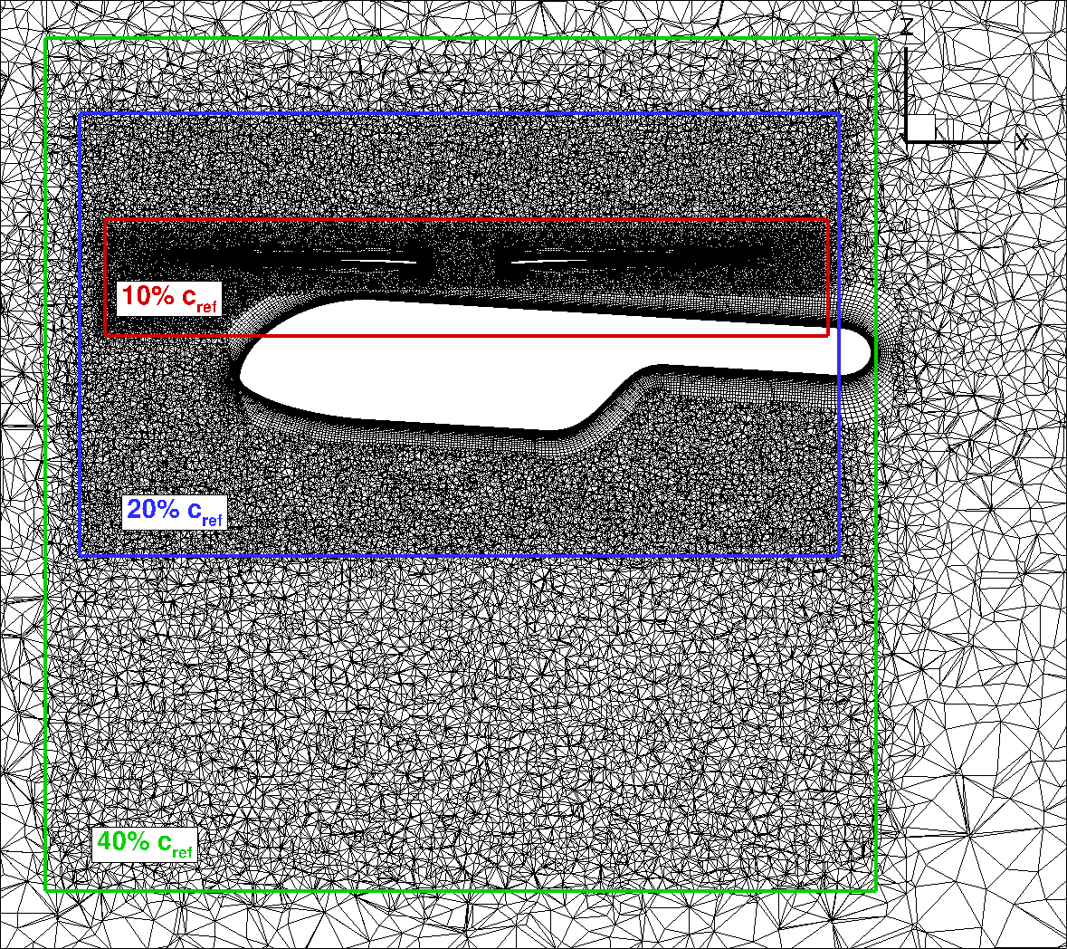
The flow in the simulation is first initialized using a 1st order solver for one revolution with a 6 degree time step, followed by 18 to 24 revolutions computed using a 2nd order solver using the same time step to establish the wake and advect the starting vortex. The simulation is continued using lower time steps, with error bars included in the integrated load results to account for long transients and low sample size. The blade was modeled as rigid, and the SA-RC-DDES turbulence model was used. The final loading results are averaged over 5 revolutions, and the confidence interval is of the same order of magnitude as the standard deviation due to the low sample size.
This concludes Part II of the series. In the next article we will discuss the results we obtained in the study and discuss their implications.
If you’d like to learn more about CFD simulations, how to optimize them, or how to reduce your simulation time from weeks or days to hours or minutes, stop by our website at flexcompute.com or follow us on LinkedIn.
For the expanded version of the paper this content is derived from, click here.
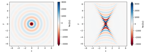
Nanophotonics is an emerging field that involves the study and application of light-matter interactions at the nanoscale. In recent years, advances in nanofabrication techniques have enabled the development of optical devices and components that are much smaller than the wavelength of light. These nanostructured devices exhibit novel optical properties that are not observed in bulk materials, making them promising candidates for a wide range of photonic applications.
In a landmark study published in Science, the lead author Dr. Peining Li from Dr. Rainer Hillenbrand’s group and colleagues report the fabrication and imaging of a mid-infrared hyperbolic metasurface based on hexagonal boron nitride (hBN). By nanostructuring a thin hBN layer into a subwavelength grating, the authors demonstrate strongly anisotropic propagation of phonon polaritons with concave, anomalous wavefronts. The results show that patterned van der Waals materials like hBN can serve as a versatile platform for hyperbolic nanophotonic devices and circuits.
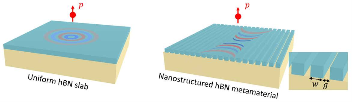
The proposed wavefront engineering for polariton waves is extremely interesting, so we replicated the simulations in the original paper and highlighted it as a public example. The simulation result is highly consistent with the prediction and experimental observation.
In addition, Dr. Peining Li has kindly agreed to do an interview with us to shed more light on their research.
What is surface phonon polariton and why does it have technological potential?
Surface phonon polaritons are a type of quasiparticle formed by the coupling of photons and optical phonons in polar crystals. They possess strong electromagnetic-field confinement, ultraslow group velocities and long lifetimes. Thus, surface phonon polaritons bear potential for various applications, including hyperlensing, directional thermal energy transfer, vibrational molecular sensing and photodetection.
How do you foresee the potential of the proposed nano-engineering techniques?
Nowadays, researchers pursue on exploring peculiar scientific phenomena on the nanoscale or even smaller scale. Thus, processing and manufacturing of nanostructures are vitally important. Based on my past research experiences, we usually rely on electron beam lithography and focused ion beam lithography to fabricate structures at nanoscale. However, such nano-engineering techniques require expensive equipment, cumbersome multistep process and harsh experimental conditions. Luckily, some patterning techniques are committed to discover the potential of the proposed nanofabrication techniques. I believe that more approaches solving existing problems can be proposed in the future.
How can fast numerical simulations accelerate research in this area?
Fast numerical simulations are of great importance and convenience to researchers in our area. Before sample fabrications, we can foresee experimental results and accordingly design complex nanostructures by numerical simulations. In addition, simulations help us to verify and check the results after experiments. In my work titled “Infrared hyperbolic metasurface based on nanostructured van der Waals materials” in Science, numerical simulations are used multiple times. They effectively present exotic wavefronts of polaritons in such a complex hyperbolic metasurface, and offer researchers a deep insight into photonic phenomena. In a word, fast numerical simulations are a powerful tool to raise efficiency of scientific research.
Can you share some of your upcoming work?
Our group is working on spatial temporal nanoimaging on hyperbolic polaritons. We are going to publish an article titled “Ultrafast anisotropic dynamics of hyperbolic nanolight pulse propagation” in Science Advance. As known to all, Scattering-type scanning near-field optical microscopy (s-SNOM) provides high spatial resolution reaching down to ~10 nm in broad spectral ranges from visible to terahertz frequencies. Our technique combines time-domain interferometry and s-SNOM, providing unparalleled imaging resolution for measuring the anisotropic propagation of hyperbolic polariton pulses. A comprehensive strategy encompassing data acquisition, processing, and interpretation has been developed to address the challenges associated with the high-dimensional spacetime.
Can you give some suggestions to students who want to work in this field?
I suggest the students who want to work in this field to think more and learn more. Students need to think more before starting a project and doing every experiment. Repeatedly confirm the meaning and purpose of projects and experiments, and make sure you fully understand the aim of every step of experiments. Once deciding to start a project and experiment, try your best to do the tasks. Learn more and devote your time to finish the tasks, so you won’t regret later.

Dr. Peining Li received his PhD in Physics from RWTH Aachen University in 2016. After working as EU Marie Sklodowska-Curie fellow at nanoGUNE in Spain from 2016 to 2019. Subsequently, he started as a full professor at Huazhong University of Science and Technology. Dr. Li’s research focuses on optical nano-imaging of light-matter interaction at extreme scales and has published numerous articles in top scientific journals such as Science and Nature.
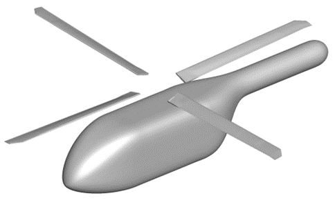
In this series of articles, we highlight our efforts to accurately model the flow physics of a hovering helicopter rotor in isolation and installed on a fuselage using the solver Flow360. In Part I, the motivation for the simulations is discussed. Part II provides details on the computational setup, including the rotor blade geometry, the Flow360 CFD solver, the treatment of turbulence, the computational grid, and the sliding interface methodology. Part III presents the simulation results, including the effect of mesh refinement and time resolution, collective sweep studies, and comparisons with experimental data and other CFD codes.
Early History and Development
Helicopters are one of the most versatile aircraft in existence, capable of hovering, vertical takeoff and landing, and flight in any direction. Nevertheless, the concept of the helicopter goes back centuries. The first recorded mention of a helicopter-like design dates back to the 4th century, when Chinese children played with bamboo flying toys that spun when a stick was rapidly twisted between their palms. The famous inventor and philosopher, Leonardo da Vinci, also imagined a helicopter like machine and drew a sketch showing a hypothetical design consisting of a spiral rotor or an “aerial screw”.
The modern helicopter, as we know it today, was developed in the 1930s and 1940s, with Igor Sikorsky being credited as the father of the modern helicopter. Sikorsky built the first practical helicopter in the United States, the VS-300, in 1939. This early design had a single main rotor and a small tail rotor to counter the yawing moment of the main rotor. Sikorsky continued to refine and improve upon his designs, culminating in the first mass-produced helicopter, the Sikorsky R-4, which was used extensively as early as World War II.
In order to design a functioning helicopter, a great deal of engineering and innovation is required. The main rotor of a helicopter is a rotating wing that generates thrust to lift the aircraft off the ground and keep it aloft. However, in order to make the conventional helicopter design functional, stable, and controllable, a tail rotor is also required. The tail rotor provides a counteracting torque to the main rotor, allowing the pilot to control the helicopter’s direction and prevent it from spinning uncontrollably. A minority of designs have counter-rotating rotors, whether in tandem, side-by-side, co-axial or intermeshing, and dispense with the tail rotor.
Additionally, the complex design of a helicopter requires a sophisticated control system to allow the pilot to manage the aircraft’s motion with six degrees of freedom. Helicopters use a combination of hydraulic, sometimes electrical, and mechanical controls to adjust the rotor blades in collective and in cyclic mode, and the tail rotor, allowing the pilot to change the helicopter’s direction and altitude. Most rotors are also articulated, initially with hinges and now often with elastic connections.
Despite the many challenges involved in designing and building helicopters and their high cost, whether initial, in maintenance or in fuel, they are widely used in a variety of fields, from military operations to emergency rescue and medical transport. Helicopters have also played a significant role in advancing scientific research and exploration, allowing researchers to access remote locations and study the natural world from new perspectives.
CFD Modeling of Hovering Rotors
Early development cycles of helicopters involved basic theories boosted by engineering judgment, followed by testing of various scale models and prototypes in wind tunnels or building working prototypes which could be tested. In the modern era, however, computer modeling has transformed the way we design and refine all aircraft. Computational modeling allows rapid performance characterization. However, despite the high degree of maturity reached by engineering-level calculations, computational fluid dynamics (CFD) codes still face challenges in accurately predicting hovering rotor performance.
CFD predictions have reached an accuracy level of within one count (0.01) in Figure of Merit (FoM). Figure of Merit is the ratio between the ideal induced power calculated from the basic theory and the actual required rotor power. Typical values in the best conditions range from 0.7 to 0.8. A higher FoM value, therefore, means lower fuel consumption and longer hover endurance, and can also mean higher max takeoff weight for a given engine power and rotor diameter.
However, some uncertainty remains about the accuracy of CFD results and the sources of contributing errors. That is, are accurate high-level results correct for the right reasons or are there compensating errors at play. In addition, a 0.5% error in FoM prediction is equivalent to the weight of a single passenger, highlighting the importance of accurate CFD prediction. Typical experimental datasets provide only a level of accuracy within 1-2 counts in FoM, indicating the need for further improvements in both computation and experiment. Engineers also deal with the FoM of the rotor being diminished by the download on the fuselage, which introduces additional difficulties; the power to drive the tail rotor is also sizable.
Hover Prediction Workshop
The Hover Prediction Workshop (HPW) has attempted to improve the accuracy and fidelity of isolated hovering rotor simulations since 2014. However, many of the issues raised in the 2017 status paper are still present in current simulations, especially for more complex problems than an isolated rotor. These issues suggest that many hover performance predictions may have good agreement with experimental data partly due to error cancellation. Only two quantities of interest are typically assessed, namely the thrust for a given RPM and blade angle, and the torque which sets the FoM. The lack of a comprehensive experimental dataset is another limitation that hinders progress in rotor-in-hover simulations. There are also “hangar effects” in testing which are difficult to model with CFD.
To address these limitations, the HPW has set a new hover focus problem, with future research planned to focus on fuselage download predictions and in-ground effect simulations of the Hover Validation and Acoustic Baseline (HVAB) rotor. While careful attempts have been made for isolated rotors in terms of grid resolution, temporal accuracy and turbulence modeling, close to no sensitivity studies exist for installed rotor predictions.
For this reason, one of the main aims of this article series is to perform rigorous mesh-refinement and time-step studies to give higher confidence in the performance predictions for both isolated and installed rotor configurations. Based on the findings from this study a collective sweep is performed for the HVAB blade. Additionally, as the HVAB blade experimental data has not yet been published, lower blade tip Mach number simulations representative of the Pressure Sensitive Paint (PSP) blade simulations are also performed. As seen in Figure 1, our CFD model is missing the rotor hub. Except for forward flight conditions when the velocities in the hub region can become substantial, we can ignore the rotor hub without greatly affecting the quality of the simulation results.
Following the earlier theme of our article series, this first part focuses on the motivation for conducting the simulations. In the second part of the series, we will provide details about the computational setup used in the study. We will present the details of the rotor blade geometry which we used for our simulations. We will also present relevant details about our CFD solver, Flow360. It is based on hardware/software co-design with emerging hardware computing, leading to unprecedented solver speed without sacrificing accuracy. We will discuss a few details about the computational grid utilized to solve such problems. For instance, we utilized the “sliding interface methodology” to simulate the motion of a rotor blade rotating around its hub; this approach helps to simulate the system more efficiently. The treatment of the tip vortices and the interaction between the rotor vortical wake and the fuselage in terms of turbulence will also be discussed.
In the last and 3rd part of the series, we will present the results obtained from our simulations. In particular, we will demonstrate the effect of changing the grid resolution on the simulation results, as well as the effect of changing the time step resolution used to resolve the movement of the rotor blades. We will then present results of a collective sweep study performed at two blade tip Mach numbers for isolated and installed rotors, and comparisons are made with experimental data and predictions from other CFD codes, where available. The Flow360 results show strong correlation with reference data and resolved high-resolution wake structures, showing the applicability of Flow360 to hovering rotor solutions.
This concludes Part I of the series. In the next article we will discuss the details of the computational model used to simulate the hovering rotor conditions.
If you’d like to learn more about CFD simulations, how to optimize them, or how to reduce your simulation time from weeks or days to hours or minutes, stop by our website or follow us on LinkedIn.
For the expanded version of the paper this content is derived from, click here.

Current technological trends emphasize the dense integration of photonic components on a chip. However, as the proximity between these components increases, the issue of crosstalk becomes more significant and detrimental. Therefore, photonic engineers need to apply other design ideas to actively minimize the crosstalk.
The research group led by Professor Sangsik Kim utilized anisotropic metamaterial cladding to achieve a remarkable reduction of crosstalk by leveraging exceptional coupling. Their novel designs have led to subsequent publications in Optica and Light: Science & Applications.
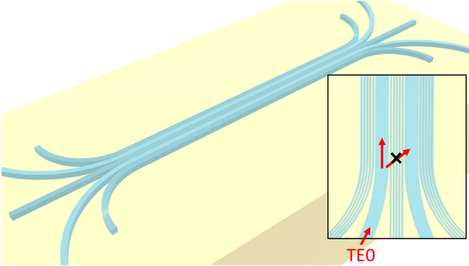
We replicated the simulations of the interesting results presented in the original paper and highlighted it as a public example. The simulation contains long waveguides (>100 µm) and fine details (the metamaterial cladding), which is challenging for conventional full-wave solvers. However, Tidy3D only took minutes to finish the job!
In addition, Professor Kim has kindly agreed to do an interview with us to shed more light on his research. Below is the full interview, containing our questions and his responses.
1. What are anisotropic metamaterials and why are they useful in integrated photonics?
Anisotropic metamaterials form a unique subset of metamaterials, which are artificially designed to exhibit exclusive characteristics not found in natural substances. Anisotropic metamaterials exhibit a strong anisotropy in their dielectric permittivity, leading to distinct εx, εy, and εz. In integrated nanophotonics, such anisotropic metamaterials can be implemented using a grating pattern whose periodicity is much less than wavelength; thus, subwavelength gratings (SWGs) serve as the primary implementation of anisotropic metamaterials. By manipulating the direction, filling fraction, and tilt angle of the SWGs, one can modify the refractive indices of the homogenized effective medium, especially tailoring the anisotropic properties. This versatile capability to adjust the effective medium is crucial in shaping the optical mode size and phase, skin-depth of a guided mode, and dielectric perturbations, thereby essential for designing various photonic device components.
2. Why is crosstalk suppression important?
Crosstalk pertains to an undesirable coupling among adjacent optical waveguides or devices, a common challenge in photonic integrated circuits (PICs). For example, suppose we place two conventional strip waveguides nearby. In that case, the optical power in one waveguide will transfer to the other (i.e., crosstalk) due to the evanescent field coupling. Consequently, one needs to separate two waveguides large enough to avoid the crosstalk, and this inherently restricts the integration density of the photonic chip, thereby limiting the scalability of PICs. Thus, crosstalk suppression is critical for achieving a more densely packed PIC, resulting in more scalable, cost-effective chips. Moreover, the degree of crosstalk is directly related to the background noise level in a PIC, which becomes increasingly significant in larger-scale PICs. Therefore, crosstalk suppression plays a pivotal role in PICs, particularly from the perspective of scalability.
3. What is exceptional coupling?
Exceptional coupling refers to an extraordinary coupling phenomenon that effectively eliminates coupling, or in other words, achieves completely zero crosstalk even between closely spaced waveguides. This significant breakthrough leverages SWGs to engineer waveguide perturbations anisotropically. For example, in a conventional strip waveguide, the perturbation is isotropic, and the coupling follows the dominant electric field and is finite. But in the case of anisotropic metamaterials like SWGs, even the other field components contribute significantly to perturbation since the perturbation strength is weighted differently (Δεx≠Δεy≠Δεz), i.e., anisotropic perturbation. Exceptional coupling represents a unique point where the total coupling coefficient equals zero (|κ|=0), achievable exclusively via anisotropic perturbation with SWG, leading to zero crosstalk. This exceptional coupling was achieved in guided TE and leaky TM modes, as detailed in Optica 7, 881–887 (2020) and Light: Science & Applications 12, 135 (2023).
4. How can fast numerical simulations accelerate research in this area?
Fast numerical simulations hold immense potential in propelling the general field of integrated photonics, including SWG anisotropic metamaterials. Faster simulations can expedite optimizing device designs and validate concepts at a larger scale, thereby significantly reducing the time and cost associated with experimental efforts. For example, while we knew about the existence of exceptional coupling in Optica 7, 881–887 (2020) via modal analysis, it took much time to verify and demonstrate it experimentally. Since our signals and phenomena occur at the noise level, we needed total device lengths larger than 100 μm, which would require a long time for full FDTD simulations. At this scale, running a few simulations to confirm the phenomena is feasible but not ideal for optimizing or more iterative works. Thus, we even did not attempt to run a full FDTD but directly worked on experimental demonstrations. We needed to run a couple of trials to demonstrate the results. However, utilizing fast simulation tools like Tidy3D could have accelerated this iterative and optimization process, reducing the time spent on the experiments.
5. Which part of the work gets you most excited?
The most exciting part of our work is the new type of waveguide coupling with anisotropic media, which is realistic and provides more degrees of freedom for modal engineering. We are excited to add new mechanisms to dielectric perturbation and waveguide coupling, which are well-established and widely used fundamentals in photonics. Moreover, these phenomena are not just academically thrilling but also hold substantial practical value. Since SWGs can be realized through periodic patterns with low-loss dielectrics, this concept has significant potential to propel industrial advancement, not limited to academic innovation.
6. Can you share some of your upcoming work?
Currently, our team is trying to apply SWG metamaterials to other component-level PIC devices to enhance their performances, including reducing noise levels and device sizes. Note that our findings on exceptional coupling were predominantly based on simple waveguide schemes and modes. We intend to extend these modal properties to other functional devices to decrease crosstalk and introduce larger birefringence. Our ultimate goal is to transform traditional PIC schemes into SWG-based PIC schemes, achieving larger scalability and reduced noise within the chip.
7. Can you give some suggestions to students who want to work in this field?
I encourage students to expand their intellectual horizons and not limit themselves to a specific research boundary. Attend conferences, interact with peers, and learn from researchers in other fields. I like Steve Jobs’ quote: “Creativity is connecting dots,” and suggest students identify and collect their own dots of knowledge. Finally, have a strong faith that those dots will eventually be connected to innovate the future, which will be.

Professor Sangsik Kim received his BS from Seoul National University in 2008 and PhD from Purdue University in 2015. After a postdoc experience at NIST, he started an Assistant Professor position at Texas Tech University and moved to an Associate Professor position at the Korea Advanced Institute of Science and Technology (KAIST) in 2022. Professor Kim’s research interest is developing novel integrated nanophotonic devices and their applications, seeking to bridge the gap between new science and future technologies.
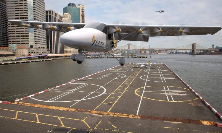

For a long time, science fiction movies have imagined aircraft navigating through skyscrapers in a bustling modern city. However, the reality is that cities lack runways for aircraft, and helicopters are too loud and inefficient for mass-market transportation. This is where Electra’s electric Short Take-Off and Landing (eSTOL) aircraft comes in.
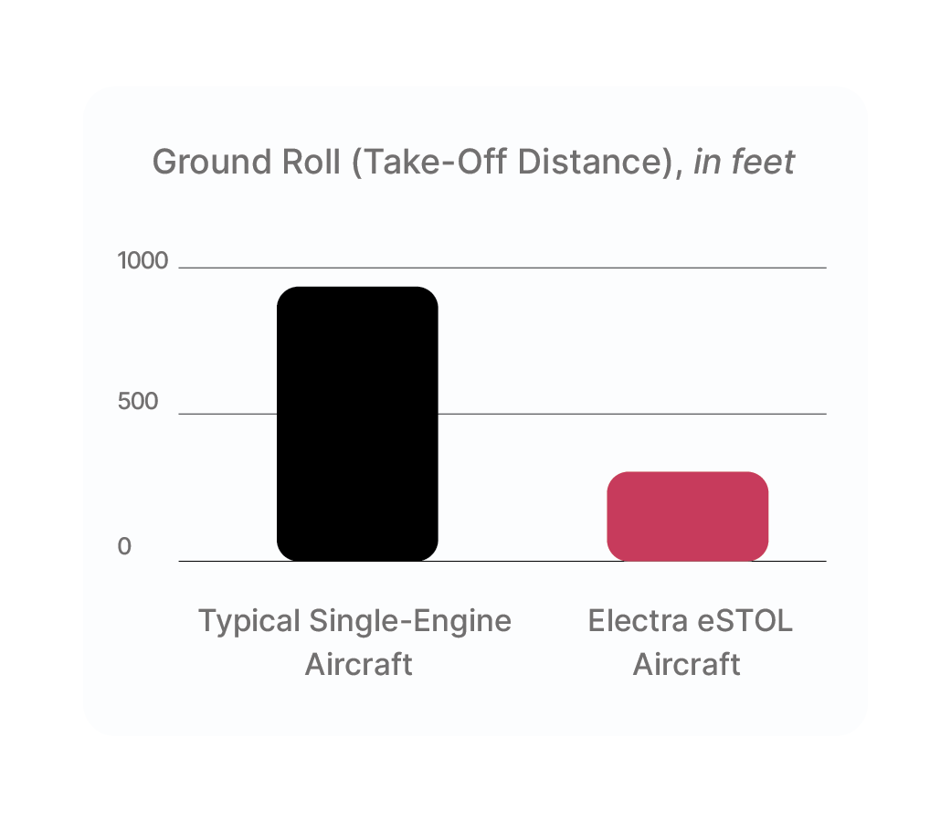
By mounting an array of propellers along the aircraft’s wingspan, Electra can achieve short take-off from urban rooftops and parking garages. These propellers are uniquely designed and positioned to create high speed airflow blowing toward the wings, which can generate extra lift force to allow the airplane to take off in a short distance. For such an innovative design, there is a lack of empirical design rules for engineers to draw from. Engineers must rely on computational fluid dynamics (CFD) simulation to design.
The challenge is the enormous design space; the size, position, and number of propellers and wings, their interaction with control surfaces, etc. There are tens of configurations that all must be simulated in each of various operating scenarios, like take-off, landing, transition, loiter, and more. And each operating scenario must be mixed with environmental effects and different performance conditions, like how much weight the aircraft is carrying or whether urgency or efficiency is the priority. Electra was quickly facing thousands of simulations to inform its overall aircraft design. What’s even more challenging is that, as a startup, Electra needs to finalize a design within a very short period.
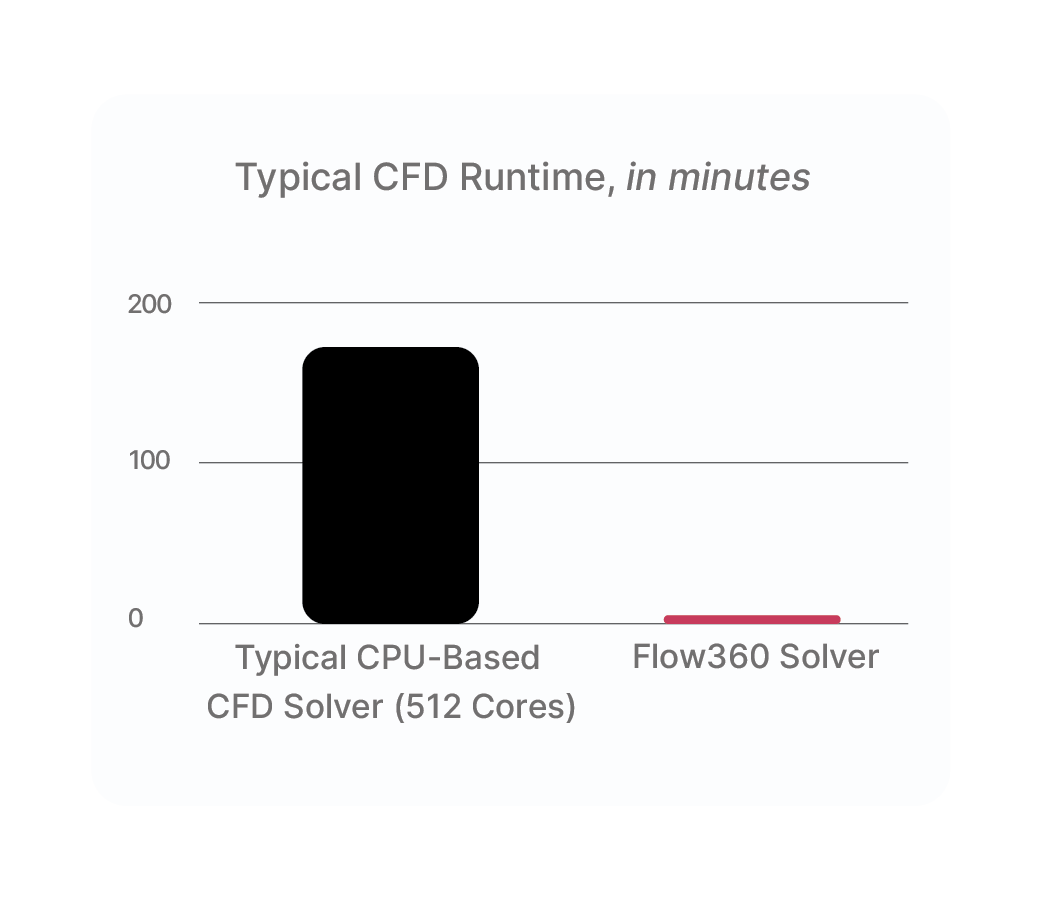
Flow360 is fast, built from the ground up for emerging computing chips, such as GPUs. Simulations that once required 3 hours to run now only require 5 minutes with this solver. Flow360 is reliable, built specifically for high-end CFD applications in aerospace and automotive, nor does it sacrifice accuracy for speed. Running Flow360 is easy, with an option to run in the cloud. Without having to maintain any computing hardware, this solver saves the Electra team hundreds of thousands of dollars.
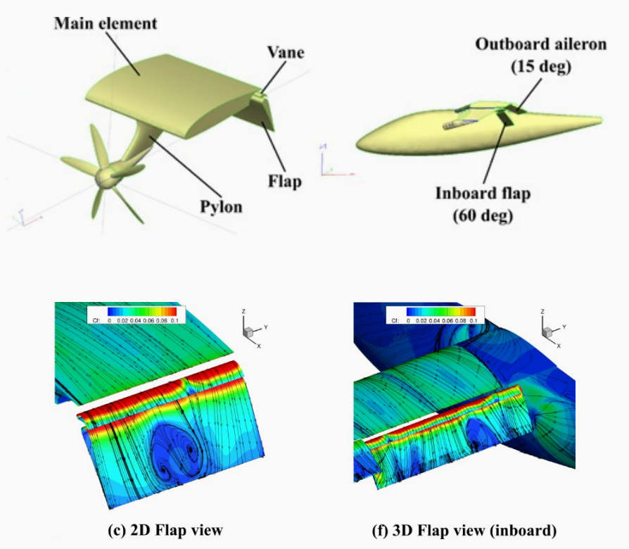
Even though Electra has some of the world’s most renowned aerodynamicists with decades of experience working with nearly all CFD tools, they quickly recognized that none of existing CFD tools can deliver the speed, accuracy, and cost that are required to get the job. Not until they found Flow360.
Thanks to the fast design iteration enabled by Flow360, Electra converged on an initial aircraft design within three months, which would have otherwise taken up to 12 months. Saving 9 months as a result sped up Electra’s path to market, which is time worth at least tens of millions of dollars to a company that is addressing an emerging market worth hundreds of billions dollars.
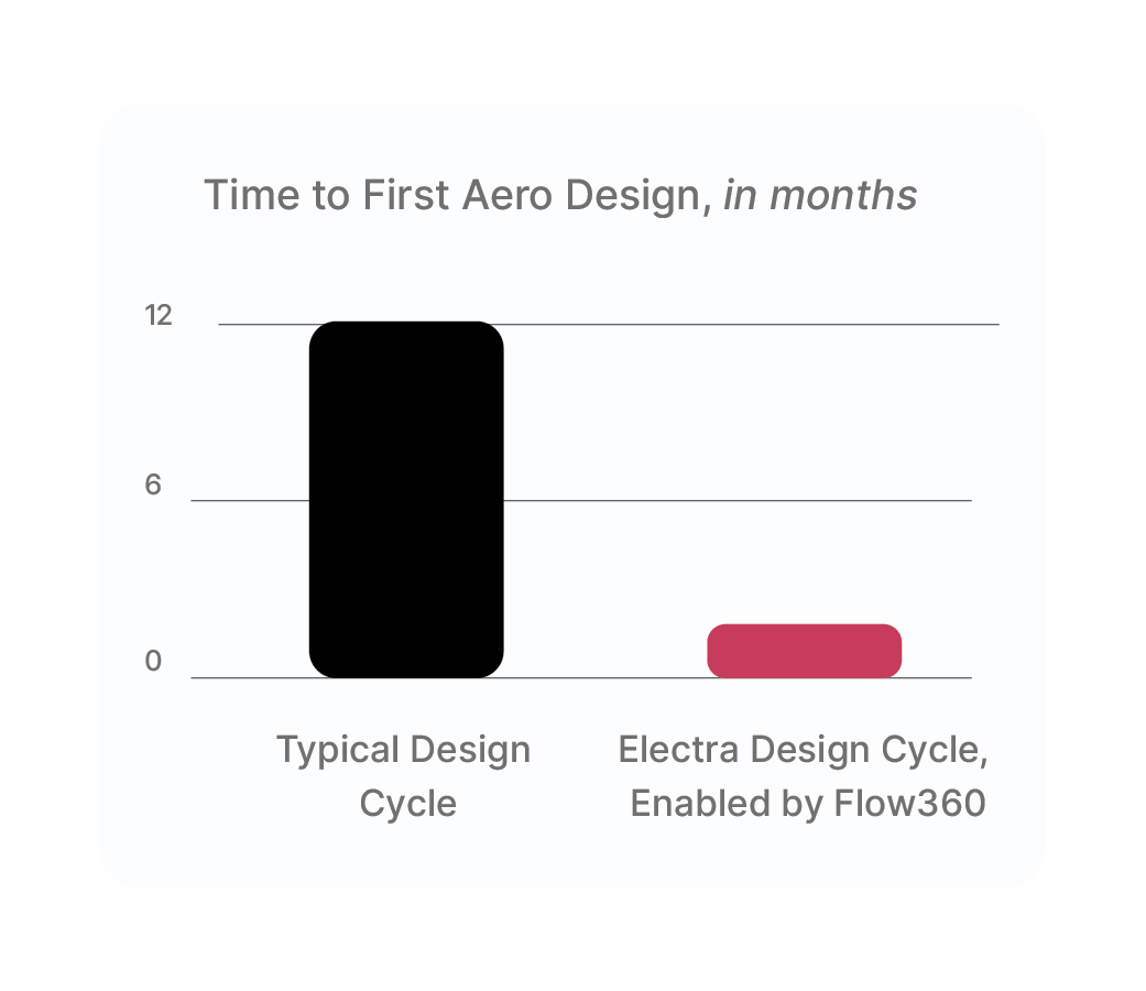
You can read more about this partnership in a paper co-authored by Flexcompute and Electra. If you’d like to learn how Flow360 enables rapid iteration in aero design, reach out to us at info@flexcompute.com and follow us on LinkedIn.
If you’ve ever tried to understand the mysteries of wave physics, you may have come across a seemingly elusive phenomenon known as Anderson localization. Proposed back in 1958 by physicist Phillip Anderson, this theory, which earned him a Nobel Prize in 1977, describes how waves behave when they encounter multiple obstacles in a disordered material. Yet despite its potential impact across fields, Anderson localization has largely remained a theoretical concept due to the complexities of confirming it experimentally and the high computational demands of simulating it.
But all of that is about to change, thanks to a team of researchers led by Professor Hui Cao of Yale University. In a landmark study recently published in the journal Nature Physics, Cao and her colleagues have managed to simulate Anderson localization using computational electromagnetics, proving Anderson’s theory and providing a potential pathway to resolving other complex physics problems.
Anderson localization is fascinating because it predicts a counterintuitive behavior of waves. When a wave—be it electromagnetic, electron, seismic, or water wave—encounters an obstacle, we’d expect it to scatter and then continue beyond the obstacle. But Anderson localization suggests that if a wave encounters multiple obstacles, it doesn’t just scatter—it bounces back and forth between the obstacles, becoming trapped, and thus, localized.
Scientists have long sought to validate this theory. Yet, the subtle signals produced in the experiments often get drowned out by statistical “noise,” making proof elusive. Moreover, simulating Anderson localization computationally is a significant challenge, requiring a large computational domain, fine resolution to resolve wave physics, and thousands of ultra-fast simulations to probe different parameters and angles.
The breakthrough arrived when Cao utilized Tidy3D with her international team, including Prof. Alexey Yamilov at Missouri University of Science and Technology, Dr. Sergey Skipetrov from University of Grenoble Alpes in France). Tidy3D is a simulation tool developed by Flexcompute, which was co-founded by Dr. Zongfu Yu, who also a senior author, and uses an algorithm for modeling electromagnetic waves based on the Finite-Difference Time-Domain (FDTD) method, an effective tool for modeling nanoscale optical devices. When coupled with advanced computing chips available in the cloud (the same chips that power AI), this tool allowed the researchers to speed up their calculations dramatically and run the simulation thousands of times. Dr. Tyler Hughes and Dr. Momchil Minkov, also from Flexcompute, contributed to this work by enabling the researchers to perform massive scale simulations.
The result? They confirmed Anderson’s theory over half a century after it was first proposed. The simulation also provided insights into why experimentalists have struggled with observing the effects of Anderson localization and proposed a non-intuitive experimental setup that could prove the theory in real-life settings.

The success of this project has far-reaching implications, as this type of computational resource could be applied to numerous other electromagnetic physics problems. “Those are just a few problems these computational methods can be used for,” Yu says. “The discoveries enabled by ever more powerful computing never fail to surprise and excite us.”
The contributions of this research extend beyond wave physics, potentially impacting fields like data center optimization and the development of nanostructured nanolenses for chip-based lidar, a remote sensing technology.
In this exciting era of computational progress, it’s thrilling to witness how powerful computing is enabling us to dive into and unlock the secrets of complex physical phenomena. The successful simulation of Anderson localization stands as a testament to the possibilities that lie ahead.
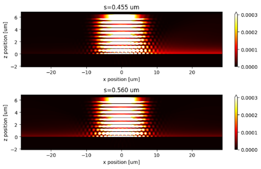
The field of non-Hermitian photonics has seen rapid growth in recent years, with new theoretical insights and experimental demonstrations being reported all the time. Recently, the research group led by Professor Yongmin Liu from Northeastern University demonstrated the precise subwavelength control of light by utilizing the exceptional point in a non-Hermitian system. This work achieved the unidirectional propagation of surface plasmon polariton (SPP) on gold film by engineering a non-Hermitian metagrating structure and has led to a publication in Science Advances recently.
We found the research to be extremely novel and interesting. Therefore, we replicated the simulations in the original paper and highlighted it as a public example. In the simulation, we controlled the geometry of the grating structure and achieved the tuning of SPP propagation direction switching, consistent with the observation reported in Professor Liu’s paper.
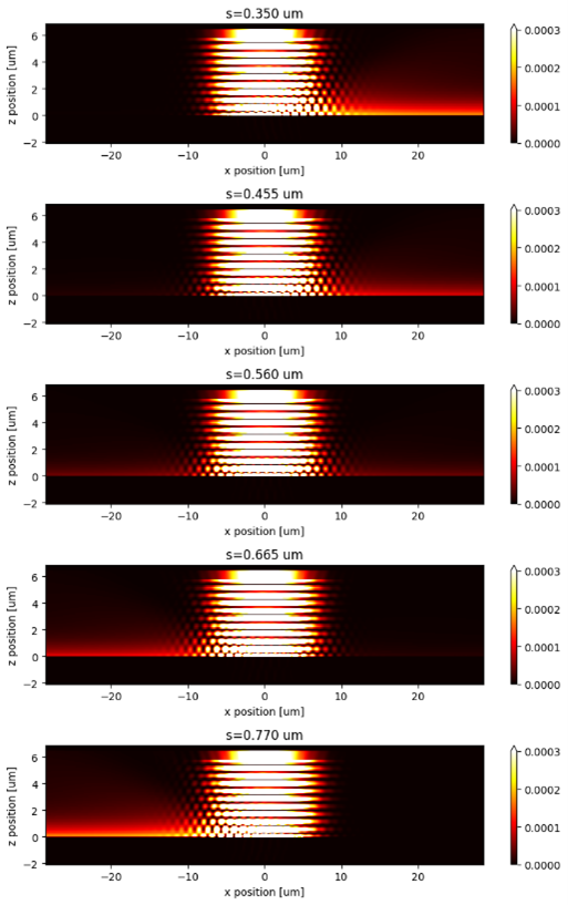
In addition, Professor Liu and the lead author of the paper, Yihao Xu, have kindly agreed to do an interview with us to shed more light on their research. Below is the full interview, containing our questions and their responses.
What is non-Hermitian photonics? Why is it interesting?
Non-Hermitian systems are open systems capable of exchanging energy, matter, or information with their surroundings by controlling gain or loss materials. Initially introduced within the realm of quantum mechanics, non-Hermitian systems can exhibit a real spectrum under specific conditions, a concept previously unforeseen until the pioneering work by Bender and co-workers (Phys. Rev. Lett. 80, 5243 (1998)). The presence of exceptional points (EPs), which are singularities where the eigenvalues of a non-Hermitian system start the transition from real to complex values, is particularly intriguing in the system. Around these EPs, novel phenomena can arise, such as mode selection, enhanced sensitivity, and robust mode propagation. However, realizing non-Hermitian behaviors in quantum systems poses significant challenges. The equivalence between the Schrödinger equation and the paraxial equation of diffraction in optics has allowed researchers to use photonic systems as an alternative platform to study non-Hermitian physics. In turn, the rich physics of non-Hermitian systems has yielded new insights and discoveries within the field of photonics.
What is an exceptional point?
EPs represent unique instances in which the eigenvalues of a non-Hermitian system undergo a transition from real to complex values. Essentially, the non-Hermitian system involves a spatial gain/loss distribution, and allows coupling between regions with gain and loss. When the gain and loss rates are low, the energy exchange between different regions through coupling is easily compensated, resulting in eigenmodes that do not display a net gain or loss. In other words, the eigenvalue is a real number. However, as the level of gain or loss increases, the energy exchange through coupling becomes incomplete. Consequently, the eigenvalues of the system begin to exhibit a net gain or loss simultaneously. The determination of the exceptional point relies on the interplay between the strength of gain or loss and the coupling in the non-Hermitian system.
Can you give some suggestions to students who want to work in this field?
First of all, it is crucial to thoroughly study the basic concepts, such as the Hamiltonian matrix, non-Hermitian systems, and the representation of parity-time symmetry in quantum mechanics. It is equally important to delve into the fundamental principles that govern EPs and understand the behaviors of eigenvalues within these systems. Rather than solely focusing on the mathematical representation of non-Hermitian systems, students are recommended to grasp the underlying physics behind them.
Once a solid conceptual understanding is achieved, the next step is to engage in simulations of real-world systems. Theoretical studies often involve various approximations and assumptions, whereas conducting full-wave simulations allows for the inclusion of practical factors. By simulating real-world scenarios, students can gain practical insights and validate theoretical findings.
Finally, it is vital to follow the latest advancements in the field. This can be achieved by regularly reading scientific papers, actively participating in conferences, and engaging with esteemed researchers and experts in the field of non-Hermitian photonics. By doing so, students can remain informed about the current trends, emerging challenges, and potential opportunities in this rapidly evolving field.
How can fast numerical simulations accelerate research in this area?
In a theoretical study of a non-Hermitian system, we usually involves a lot of assumptions and approximations, like tight-binding and effective medium models. However, we need to consider all physical factors and constraints that may exist in experimental measurements, and quite often, we need to sweep the parameters for an optimal device design. In a brute-force search of the optimal design, the time cost is exponentially scaled with the number of parameters involved. Using an optimization algorithm can speed up this process but not by orders of magnitude. Therefore, a fast numerical simulation can greatly accelerate the research especially when parameter sweeping is required.
Which part of the work gets you most excited?
The most significant excitement of this work is the translation from theory to successful experimental demonstration. In collaboration with Prof. Jing Chen at Nankai University, we published the theoretical work in 2017 (Phys. Rev. Lett. 119, 077401 (2017)) that predicted the unidirectional, radiative-loss-free excitation of surface plasmon polaritons (SPPs) based on an ideal sinusoidal permittivity distribution. However, the original design was too ideal and impractical to realize experimentally. After a long time of investigation, we conceived the idea of using two discrete meta-gratings to form a pair that could manipulate the real and imaginary permittivity. In collaboration with Prof. Junsuk Rho’s group at Pohang University of Science and Technology, we finally fabricated the device and performed experimental measurements. To our delight, the experimental results show excellent agreement with our theoretical predictions and numerical simulations. Our work pushes non-Hermitian photonics to the nanoscale regime and paves the way toward high-performance plasmonic devices with superior controllability, performance, and robustness by using the topological effect associated with non-Hermitian systems.
What are you working on? Can you share some upcoming work?
Currently, we are investigating the intriguing interplay between topology features and non-Hermitian systems, which has gained significant attention in the community. In the Science Advances paper, we have reported the analysis of the topology properties surrounding the EPs. It is shown that opposite topological charges exist at the two EPs in the non-Hermitian system. This result is related to the enhanced robustness of the unidirectional excitation of SPPs observed in our system. Our ongoing efforts target a comprehensive understanding of the underlying connections between non-Hermitian systems and topological photonics. Furthermore, we are actively investigating methods to manipulate and control topology features in non-Hermitian systems. We hope to unveil new possibilities for harnessing their unique properties in advanced photonic applications.

Dr. Yongmin Liu obtained his Ph.D. from the University of California, Berkeley in 2009. He joined the faculty of Northeastern University at Boston in fall 2012, and currently he is an associate professor in the Department of Mechanical & Industrial Engineering and the Department of Electrical & Computer Engineering. Dr. Liu’s research interests include nano optics, nanoscale materials and engineering, plasmonics, metamaterials, biophotonics, and nano optomechanics.

Lumotive is a technology startup based in Redmond, Washington. It is a leading developer of optical semiconductors which are changing the rules for LiDAR across a wide range of 3D sensing applications. Their proprietary Light Control Metasurface (LCM™) solid-state beam steering chips are manufactured using proven and scalable CMOS semiconductor processes and eliminate the need for mechanical moving parts. This significantly reduces the complexity, cost, size, and power consumption of 3D sensing systems, while improving both performance and reliability.
Modeling the LCM chips is inherently challenging due to their large aperture and small subwavelength structures. Full-wave electromagnetic simulations are required to accurately capture their behavior.
 technology for next-generation LiDAR systems from Lumotive")
In 2022, Dr. Laura Pulido-Mancera joined Lumotive’s R&D team after the company had already delivered its first-generation beam steering chip prototype. Laura was tasked with designing the second-generation beam steering device to increase efficiency. With over 8 years of experience in modeling and designing metamaterial antennas, Laura identified several design parameters that might impact the device’s performance. However, she soon realized that their existing simulation tool was insufficient to effectively search the entire parameter space.
A proper and systematic parameter sweep study would need to cover multiple design parameters concurrently to generate meaningful insights. This could easily result in hundreds to thousands of simulation runs, making it impossible to accomplish with the existing simulation tool within an acceptable time frame.
Specifically, Laura and the rest of the R&D team had an intuition that making certain geometric and material changes could significantly improve the efficiency of the device. However, they lacked the computing resources with existing simulation tools.
Fortunately, Laura discovered Tidy3D just in time. With Tidy3D’s super-fast simulation speed, she was able to run full parameter sweep batches and validate the hypothesis that making the proposed changes could significantly improve device efficiency. Laura’s simulation results were instrumental in enabling the team to make the critical in changing the manufacturing process. As predicted by Tidy3D’s simulation results, this move increased the device efficiency substantially.
Guided by Laura’s simulations, the R&D team gained confidence in their technical decisions, which helped them tune other geometric parameters. This ultimately will lead to the delivery of Lumotive’s second-generation LCM chips, a significant milestone in the company’s technological achievements.
“Tidy3D has been an amazing tool for Lumotive. Saving months of time in simulations is crucial for the decisions we are making as a company. We are using the results from Tidy3D for our next-generation metasurface!”
— Dr. Laura Pulido-Mancera
One of Lumotive’s strategic goals is to lead the industry toward “LiDAR 2.0”: the next generation of LiDAR featuring modules built with solid-state components which can be integrated into any system as easily and pervasively as 2D cameras are today. This means that the platform needs to be flexible and adjustable to a wide range of sizes, prices, performances, and power requirements, from the high-performance, long-range solutions demanded by the automotive industry all the way down to the ultra-small form factor and low-cost solutions needed for smartphones. This poses extremely high requirements on the performance, uniformity, and reliability of Lumotive’s core LCM chip.
Traditionally, sensitivity analysis and optimization of uniformity and reliability required fabricating batches of test wafers and conducting measurements. However, these experiments are expensive and time-consuming. In some cases, the team had to skip them and take the risk.
After Laura used Tidy3D to perform high-throughput sensitivity and corner analysis, she was able to optimize the design so that the manufacturing team didn’t have to fabricate as many test wafers as before. This saved the company tens of thousands of dollars and months of development time. As a result, the LCM chips have higher efficiency, can reach further distances, and integrate better at the system level. Tidy3D allowed Lumotive to gain an advantageous position in the “LiDAR 2.0” race.
By converting qualitative “intuition” into quantitative “prediction” and extracting valuable insights from simulation data, Tidy3D empowers design engineers to confidently steer the direction of research and development.
Are you a design engineer like Laura who is trusted by your team with critical yet challenging design problems? Reach out to our expert team to see how Tidy3D can help you, too!
The REGENT Seaglider
REGENT’s“seaglider” is a fully electric vehicle that utilizes a blown wing and hydrofoils for takeoff from the water, instead of gas powered engines and a hull used by traditional seaplanes. Seagliders are a much more efficient alternative to traditional hopper flights and a much faster alternative to traditional ferry routes. Such an efficient commuter transport will be greatly beneficial for passengers traveling between coastal cities.
Design with Detailed Flow Insights
While flying in ground effect, the seaglider’s aerodynamics are important for precise flight control capability, passenger comfort (acoustics, vibration) and safety. Addressing these design challenges requires leveraging a world class aerodynamics group using state-of-the-art simulation technologies. A revolutionary CFD solver like Flow360 provides a distinct advantage for REGENT’s engineering staff, enabling them to analyze more complex flight conditions and flow physics in significantly less time.
Our experience working with the Flow360 team has been collaborative and responsive to our fast design mentality at REGENT pushing the state of the art with speed and accuracy. Couldn’t be happier with this new simulation technique.
Bryan Baker Chief Engineer Vehicle Physics
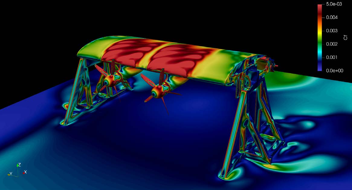
Successful Prototypes from Digital Designs
Building on a successful design process, REGENT is continuing to emphasize both digital and physical testing for their first full scale human operated vehicle, Paladin. To ensure accuracy and build correlations involving digital simulation results, REGENT is validating CFD methodologies with wind tunnel tests of a full-scale segment of their blown wing. Instrumentation onboard the test article reads surface static pressures, motor torque and power, as well as all body forces and moments. By correlating the same geometry and operating conditions both in the wind tunnel and in CFD, REGENT can increase certainty in digital designs and achieve success with its first prototype builds.
Simulation results with Flow360 are achieved in less than 6 hours. The model has more than 150M elements and is run with as little as 1° of rotation per time step for more than 25 revolutions.
By leveraging Flow360’s unprecedented speed and accuracy, REGENT engineers are able to simulate complex flows with confidence and in record time. The resulting flow insights allow for confirming assumptions, preemptively addressing concerns, and preparing for successful test campaigns.


Leading a project to optimize photonic device design, Dr. Sean Sullivan, CTO at memQ Inc., was hampered by slow photonic simulation solutions, which slowed the chip design, fabrication, and testing cycle time. As a startup developing new quantum photonic hardware for long-distance distributed quantum information, memQ was time and resource-limited and running simulations on their local machines was suboptimal. They were looking for a more efficient way of quickly tweaking and testing new designs.
After hearing positive feedback from colleagues, Sean implemented a new set of simulations and designs using Tidy3D, an electromagnetic simulation software product by Flexcompute. Tidy3D’s fast and web-based simulations helped memQ test out designs and get quick feedback on their design cycle. They were also able to avoid investing in building their own computational infrastructure, such as managing their own cluster or building multiple workstations, or even having to install any software.
Sean and his team find value especially in Tidy3D’s adjoint optimization feature, which helps tackle one of the biggest challenges that quantum photonics is facing—reducing photon loss. They are excited that Tidy3D continues to add more features to this package, which can enable new paradigms for photonic device design.
Sean appreciated how the Tidy3D team responded to the needs of startup customers like memQ, which are racing to market with new solid-state hardware designs. He found it reassuring to work with a company that could implement features and changes quickly, something that might not be possible with a larger simulation provider.
Tidy3D’s cloud-based approach to software saves companies like memQ from having to own and operate computing hardware, all while spending 10-100x less time waiting for simulation results. Lower costs and quicker design insights are gamechangers for memQ, shifting their focus from administering complex legacy simulation tools toward enabling our quantum future.
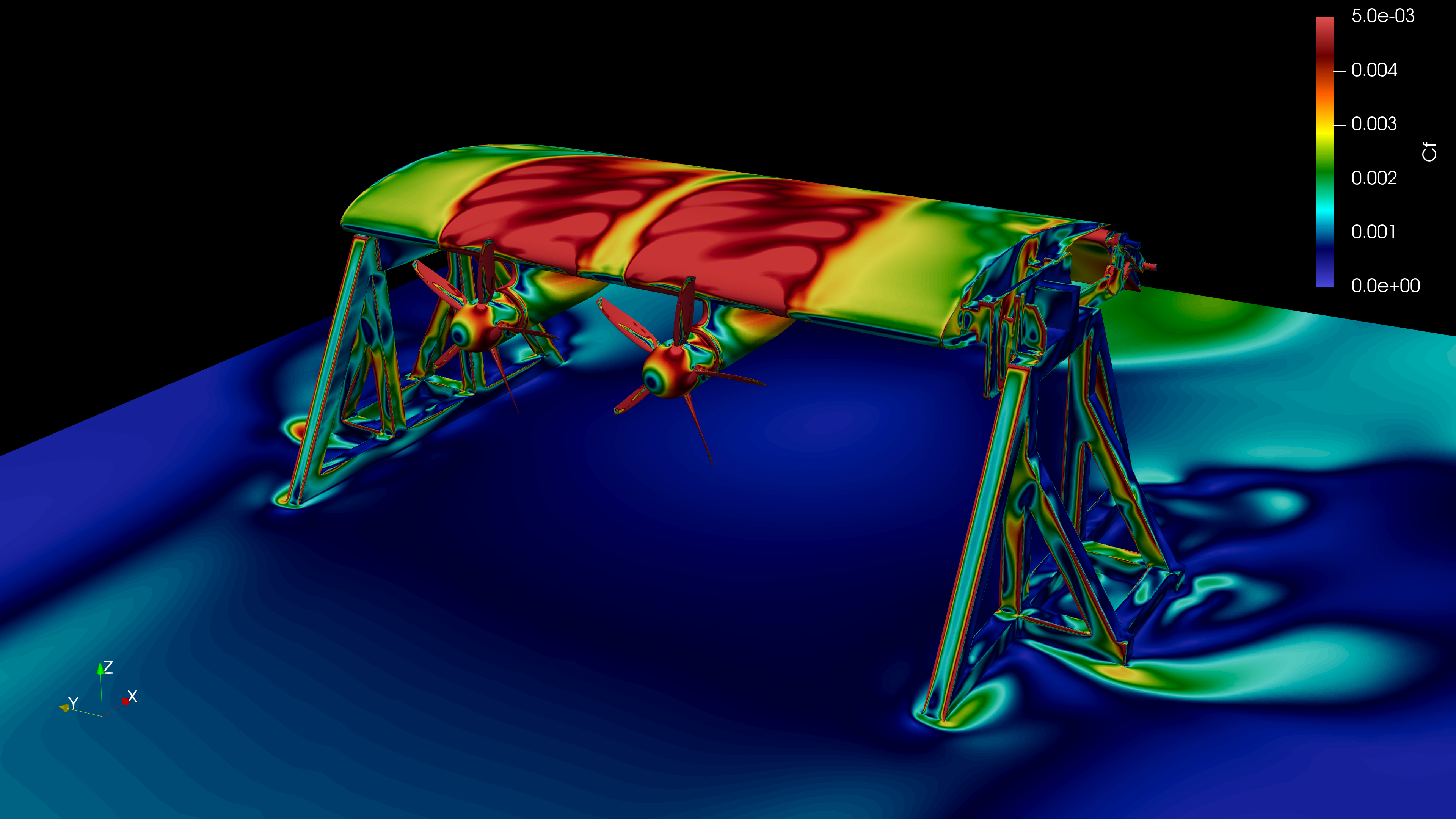
REGENT, a pioneer of zero-emission regional coastal transportation, has teamed up with Flexcompute to develop their revolutionary floating, foiling and flying “seagliders”. By leveraging our game-changing CFD solver, Flow360, REGENT engineers are able to simulate complex flow physics with greater confidence and in record time.
Introduction
REGENT, a North Kingstown, Rhode Island based company, is designing and building “seagliders”. REGENT’s seaglider is a fully electric vehicle that utilizes a blown wing and hydrofoils for takeoff from the water, instead of gas powered engines and a hull used by traditional seaplanes. Once airborne, the seaglider flies within a wing span of the water surface as a wing-in-ground-effect to take advantage of the cushion of air that forms between the vehicle and the water surface, improving efficiency. Such an efficient commuter transport will be greatly beneficial for passengers traveling between coastal cities. Seagliders are a much more efficient alternative to traditional hopper flights and a much faster alternative to traditional ferry routes.
By using electric power instead of fossil fuels, REGENT can efficiently distribute power to many motors along the wing. This not only increases the safety by adding redundancy to the propulsion system but also allows for effective blown-wing technologies. By blowing the propeller wash over as much of the wing as possible, seagliders can takeoff at much lower speeds than conventional seaplanes.
Developing such a concept combining many new technologies is a very ambitious endeavor. To develop their revolutionary floating, foiling, flying seagliders, REGENT is using computational fluid dynamics (CFD) simulations to better assess safety, performance, control, and passenger comfort criteria. By leveraging the Flow360 CFD solver at various stages of the design process, REGENT engineers are able to efficiently analyze design iterations with greater confidence.
Flexcompute’s Flow360 CFD solver ushers in a new era for engineers developing high accuracy flow solutions. By rewriting the solver from scratch using 21st century numerical methods and combining it with the latest computing technologies, Flow360 can achieve unprecedented speeds and increased accuracy. Flow360 users can do in minutes what would previously take hours or even days. The cloud computing environment scales for extremely large simulations and enables parallel throughput of extensive case matrices, all at a reduced cost.
Faster, more accurate CFD enables better development
The original seaglider concept was sketched on a napkin and quickly progressed through low-fidelity performance validations. Then detailed design work on a scaled demonstrator (Squire) was followed by coupled CFD and wind tunnel testing, leading to Squire’s successful first flight. Building on this successful design process, REGENT is continuing to emphasize both digital and physical testing for their first full scale human piloted vehicle, Paladin.
With regards to safety, the company is hyper focused on meeting or exceeding the same risk-based safety levels that are applicable to passenger aircraft. While flying in ground effect, the seaglider’s aerodynamics are important for precise flight control capability, passenger comfort (acoustics, vibration) and safety. Addressing these design challenges requires leveraging a world class aerodynamics group using state-of-the-art simulation technologies. A revolutionary CFD solver like Flow360 provides a distinct advantage for REGENT’s engineering staff, enabling them to analyze more complex flight conditions and flow physics in significantly less time.
Rotor modeling with blade element theory and moving reference frames are fast and efficient simulation techniques for initial design iterations and sizing studies, but when designing blown wings, a fully time-accurate, scale-resolving simulation with rotating mesh is preferred. The resulting pressures extracted can then be assessed by the structures team to digitally validate designs over many flight conditions before proceeding to physical testing. This enhances safety of the final product by understanding rotor-wing interactions before ever stepping into a wind tunnel.
To ensure accuracy and build correlations involving digital simulation results, REGENT is validating CFD methodologies with wind tunnel tests of a full-scale segment of their blown wing. Instrumentation onboard the test article reads surface static pressures, motor torque and power, as well as all body forces and moments. By correlating the same geometry and operating conditions both in the wind tunnel and in CFD, REGENT can increase certainty in digital designs and achieve success with its first prototype builds.
Evaluating test requirements with CFD
Preemptive CFD simulations of the wind tunnel setup can provide additional flow insights prior to the physical test campaign. Simulating the blown wing test article operating within the wind tunnel helps to reduce risk associated with the apparatus design and to inform the envisioned run matrix. Accurate and reliable CFD is used to confirm certain assumptions and answer key questions:
- This blown wing configuration is designed to generate more lift than a conventional wing of similar size. Because of this extra lift, the test stand (i.e., structural supports holding the test article) requires careful design considerations to ensure that it can handle the forces and moments generated during testing with safety margins applied.
- Testing could potentially result in significant vibrational loads and unexpected twisting/bending due to the complex flow physics induced by the model. Simulation allows for the recognition of and evaluation of unexpected response behaviors that could present safety concerns if unaccounted for.
- The test stand itself may also induce unfavorable flow conditions that could affect the quality of wind tunnel measurements. For example, the support structures and measurement equipment may disrupt the flow field near critical regions of the test article, potentially distorting measurement.
- A full-scale model poses additional challenges as its size relative to the wind tunnel test section could influence the intended operating conditions. Some of the desired test points may not be achievable due to blockages imposed by the full-scale model. The surrounding wind tunnel geometry may even affect sensitive measurements at the wing section.

Simulating the blown wing wind tunnel test
To address the above wind tunnel test considerations and develop digital-physical correlations, REGENT engineers are simulating the test configuration with Flow360. As seen in Figure 2 the test article itself includes structural supports, mechanisms for flap deflections, and two rotating propellers. Additionally, the entire wind tunnel is modeled including test section details, plenum and diffuser with turning vanes (see Figure 3).

The analysis strategy targets a series of time-accurate delayed detached eddy simulations (DDES) at various operating conditions. An unstructured mixed element mesh is generated with y+ ≤ 1 wall spacings throughout and sliding interfaces enclosing the propeller rotational domains. In total, about 4M surface elements and more than 150M volume elements comprise the CFD model.
To most efficiently simulate this complex configuration, REGENT first runs steady-state cases to initialize the flow field. Then, from these initialized conditions, a cascade of transient DDES cases are run spanning more than 25 propeller rotations. The time-accurate DDES simulations are sequentially refined to as little as 1° of propeller rotation per time step. Both the extended time period and small time step size create an accurate representation of the flow physics involved.
Flow360’s state-of-the-art performance allows REGENT to simulate these large and complex models in less than 6 hours and at a lower cost than comparable CFD solvers. The speed and accuracy provided enables engineers to make decisions based on flow insights gained from challenging problems.
Conclusion
By leveraging Flow360’s unprecedented speed and accuracy, REGENT engineers are able to simulate complex flows with confidence and in record time. The resulting flow insights allow for confirming assumptions, preemptively addressing concerns, and preparing for successful test campaigns.
REGENT is just beginning to scratch the surface of possibilities for next generation vehicles. More design concepts, wind tunnel models, and flight testing campaigns are on the horizon. Flow360 continues to expand capabilities, improve robustness, and dramatically increase performance. The solver is purpose-built and developed to empower engineers in all aspects of the design process.
In our next article we will investigate how CFD results compare to physical tests in the wind tunnel and share lessons learned about the effective application of CFD. Stay tuned.
If you’d like to learn more about CFD simulations, how to optimize them, or how to reduce your simulation time from weeks or days to hours or minutes, stop by our website at flexcompute.com or follow us on LinkedIn.
A PDF version of this article is available for download here.
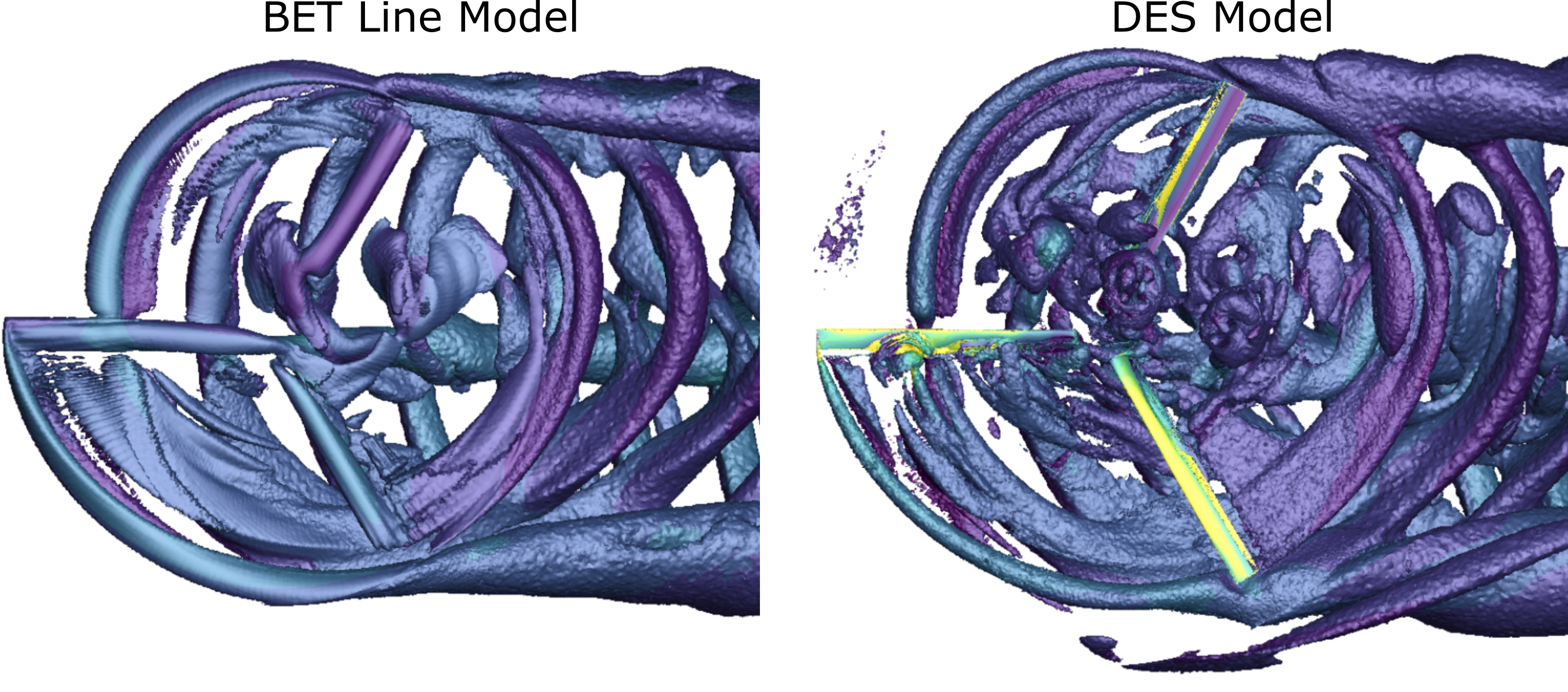
In this series, we highlight our continued effort to study the fluid dynamics of the XV-15 tiltrotor aircraft. The full series consists of three parts: Part I provides some background on the need and utility of tiltrotor aircraft and summarizes the CFD study we carried out in 2021 using the Detached Eddy Simulation (DES) technique. Part II will discuss useful fluid dynamic propulsion approximations to model the XV-15 at a reduced computational cost. Part III will showcase the results obtained using the propulsion approximations.
##
In this final article of the series, we summarize the important results obtained when modeling the XV-15 isolated rotor in various configurations using Blade Element Theory (BET).
Model specifics
Before we move on to the results, let us briefly summarize a few key aspects of the simulations. The simulations were run in three modes as described in Table 1. In the Airplane mode, the propellers face forward, while in the Hover mode they are oriented facing up. For the Helicopter mode, the propellers are slightly tilted, providing lift as well as thrust.
Two meshes were used to generate the results, one for the propeller and hovering condition, and another for the helicopter condition. The helicopter configuration involves more complex physics; therefore we generated a larger mesh refined near the rotor to better resolve the wake and the blade-vortex interactions (in BET Line mode).
The lift and drag polars for the airfoil sections of the propellers were predicted using XFOIL assuming a chord Reynolds number of 5 million.
| Hover | Helicopter | Airplane | |
|---|---|---|---|
| Mtip | 0.69 | 0.69 | 0.54 |
| Re | 4.95e6 | 5.65e6 | 4.50e6 |
| θ75 | 0°, 3°, 5°, 10°, 13° | 2° to 10° | 26°, 27°, 28°, 28.8° |
| ⍺ | - | -5°, 0°, 5° | -90° |
| 𝜇 | - | 0.170 | 0.337 |
| nodes | 2.3M | 4.1M | 2.3M |
Effect of mesh refinement
We begin by performing a mesh refinement study. The results obtained from the BET Disk model at various mesh resolutions are compared against the DES results in Figure 1.

Figure 1: Behavior of total and sectional thrust for different mesh sizes.
The data shows that the thrust is relatively insensitive to the mesh coarseness. There is a 0.6% difference in the converged thrust between the finest and coarsest mesh. Furthermore, in the right panel, the 592K node grid shows little difference in loading compared to the finer mesh. However, we decided to run all cases using the finest grid since each case only requires a few minutes of runtime due to the speed of Flow360.
Airplane mode
Let us first discuss the Airplane mode where the blades are tilted fully forward. This should be the easiest operating condition to accurately simulate since in contrast with hover there is no blade and tip-vortex direct interaction.
We compute the steady-state solution using the BET Disk method, and use the BET Line method to compute the transient solution. The BET Disk simulations typically converge within 600 pseudo steps. The BET Line simulation is run for 10 revolutions, with a time step corresponding to two degrees per step. The forces stabilized well after 10 revolutions. Figure 2 shows the torque coefficient, CQ, and propulsive efficiency, η, as a function of thrust coefficient, CT.

Figure 2: Behavior of CQ and η as a function of the thrust coefficient CQ. The four points for each model are calculated at θ75 of 26°, 27°, 28°, 28.8°.
The data shows good agreement between both BET models as compared to the high-fidelity DES results. The BET Disk method slightly over-predicts both thrust and torque compared to the DES, whereas the BET Line method under-predicts both thrust and torque. Furthermore, the BET Disk method over-predicts efficiency, η, compared to both experiment and DES, while the BET Line method predicts efficiency between the experiment and DES. All modeling approaches generally align with trending of the experimental results.
Figure 3 shows the sectional thrust loading for all pitch conditions simulated in airplane mode.

Figure 3: Behavior of sectional thrust and torque loading for different cases in Airplane mode.
The steady-state BET Disk method severely over-predicts the thrust loading near the tip, whereas the transient BET Line method tends to under-predict the thrust loading in the mid-blade region compared to DES. A similar trend persists in the case of the torque loading. The BET Disk issue is plausibly due to its failure to incorporate the tip vortex of the preceding blade, as seen in a figure from Part 2. That vorticity is instead represented simply by an axisymmetric vortex sheet.
Hovering mode
The hovering flight condition presents even more of a challenge for lower-fidelity methods, since there are often blade-vortex interactions and highly three-dimensional effects. Figure 4 shows the variation of Figure-of-Merit (FoM), calculated as a ratio of (CT)3/2 and CQ√2, as a function of CT for the hovering condition.

Figure 4: Variation of Figure-of-Merit versus the thrust coefficient for Flow360, earlier simulations, and experimental data.
The BET Disk method over-predicts the FoM by as much as 10% (due to under-prediction of the torque). The BET Line method also slightly over-predicts efficiency at lower blade loadings, but is in line with the high-fidelity and experimental efficiency for larger blade loadings.
The sectional thrust and torque loadings shown in Figure 5 reveal very good agreement in sectional thrust loading between the BET Line and high-fidelity DES methods. The surge at about 90% radius is attributed to the vortex from the preceding blade. At higher blade loadings, differences appear near the tip, in the last 20% of the blade. Again, BET Disk maintains high local loading essentially all the way to the tip.

Figure 5: Behavior of sectional thrust and torque loading for different cases in Hovering mode.
Notably, the BET Disk method over-predicts the thrust at the blade tip. The BET Line method is more in-line with the DES loading, although it tends to under-predict the thrust coefficient around 85% radius. This mismatch is caused by the highly three-dimensional nature of the flow in that region, due in part to the leading blade’s tip vortex strongly interacting with the blade.
As for the sectional torque loading for the three methods, again reasonable agreement is seen between all models for lower blade loadings. However, for higher loadings, both the BET Disk and BET Line under-predict torque, especially at r/R > 0.5. A possible reason for the under-prediction of torque in this region is the use of incompressible airfoil polars in the BET lookup tables. Although, we cannot consider the DES results to be perfect; it is only our most complete description.
Helicopter Mode
The most challenging condition to simulate is the Helicopter mode due to the complex blade-vortex interactions. This flight condition is characterized by a forward velocity with the axis of rotation close to perpendicular to the forward velocity, but typically with some incidence angle, α. A positive alpha results in the freestream flow entering the disk from below, and is typical of a descending condition. A negative alpha results in the freestream entering the disk from above, as is typically the case for level forward flight or ascending flight.
As shown in Figure 6, the BET Disk method again underpredicts CT and CQ significantly compared to experiments and DES, although CQ to a greater extent. The BET Line method predicts slightly less thrust than the BET Disk method, but the torque is closer to high-fidelity results, especially for smaller pitch angles. The agreement between DES and BET Line is close to engineering accuracy. These trends persist in the α = 0° and 5° cases (not shown).

Figure 6: CQ as a function of CT for Flow360’s DES and BET models. Also shown are existing experimental data. The α is -5° and the different data points for each model correspond to several pitch angles.
The blade thrust and torque loading distributions were compared to assess differences between the BET Line model and the high-fidelity DES results. It can be observed in Figure 7 that there is a discrepancy along the inboard section of the blade. This area of the blade is subject to large degrees of radial flow in DES, which may not be accurately modeled by the BET Line method. The behavior was similar for the sectional torque coefficient Cq.

Figure 7: The distribution of Ct along blade 1 in Helicopter mode.
Flow in BET Line vs DES
Finally, let us visualize the 3D flow field around the rotor blades in the case of BET Line and DES models to visually compare the two approaches.
 and θ<sub>75</sub> = 10°.")
Figure 8: Q-criterion isosurface comparison of Flow360’s BET Line and DES simulations. The simulation was performed at α = -5°(forward flight possibly with climb) and θ75 = 10°.
Figure 8 shows that the shed vortices interact with the other blades and convect downstream very similarly between the two methods. The forward blade clearly cuts the vortex of the preceding blade. There are differences in the vortex structures near the blade root; however, this region of the rotor has only a small effect on overall rotor performance due to its low rotational velocity. The vortices are thinner with DES, thanks to a smaller eddy viscosity.
Conclusions
We arrive at the following important conclusions after our analysis of the BET and DES modeling of XV-15:
1. Both the BET Disk but especially the BET Line methods show good agreement in terms of CT and CQ with both experimental data and previous high-fidelity CFD results.
2. Accuracy of the sectional loading coefficients for BET methods compared to high-fidelity DES shows some discrepancies, especially near the tip where the flow is highly three-dimensional.
3. The runtime for the BET Disk method is approximately two orders of magnitude lower than that for a full DES run, while the runtime for BET Line is approximately one order of magnitude less than high-fidelity. Therefore, each of these BET methods offers a good compromise between accuracy and cost, and may be favored at different stages of the design cycle.
This concludes our series of articles on the efficacy of Blade Element Theory in simulating the XV-15 rotor! It is clear that we can use the BET modeling approach to achieve tremendous savings in computational time without compromising the accuracy of results substantially.
If you’d like to learn more about CFD simulations, how to optimize them, or how to reduce your simulation time from weeks or days to hours or minutes, stop by our website at Flexcompute.com or follow us on LinkedIn.
For the expanded version of the paper this content is derived from, click here.
In this series, we highlight our continued effort to study the fluid dynamics of the XV-15 tiltrotor aircraft. The full series consists of three parts: Part I provides some background on the need and utility of tiltrotor aircraft and summarizes the CFD study we carried out in 2021 using the Detached Eddy Simulation (DES) technique. Part II will discuss useful fluid dynamic propulsion approximations to model the XV-15 at a reduced computational cost. Part III will showcase the results obtained using the propulsion approximations.
##
In the first part of this series, we discussed the utility of the Detached Eddy Simulation technique to model an XV-15 tiltrotor and similar aircraft. We found a very good agreement between the results obtained using our Flow360 solver and the available experimental results and earlier simulation studies. In this part, we discuss in detail a few propulsion approximations which can be used to dramatically cut the computational cost of simulating an aircraft involving a rotor system, compared with a simulation employing a body-fitted rotating grid on the blades.
Modeling the movement of fluid around propellers can be a difficult task for computers. The high rotation speeds and narrow blades of propellers can create very fast and complex interactions among the fluid flows associated with each blade. However, many scientific and engineering problems can be simplified with mathematical models. This allows us to understand the important physics of the problem while using fewer computational resources, making industrial studies more efficient.
Over the years, researchers have shown that the complex fluid dynamics of propellers can be approximated by simpler models. Let us discuss two appropriate models: the transient Blade Element Theory (BET Line) and the steady Blade Element Theory (BET Disk). These models make assumptions about the physics of the problem to simplify the calculations.
Propulsion approximations
The Blade Element Theory (BET) model is a significant improvement over the Actuator Disk (AD) model. Let us first discuss the AD model to lay down some basic ideas.
The Actuator Disk (AD) model is a simplified method used to model the fluid dynamics of rotor propulsion systems such as wind turbines or helicopter rotors. In this model, the individual blades of the rotor are ignored, and the entire rotor is modeled as an effective disk. The disk is assumed to take in fluid from the upstream side, perform mechanical work, and push out the accelerated fluid from the downstream end.
This simplification allows for the calculation of the rotor’s influence on the flowfield using only two parameters: the axial force, or “thrust”, directed along the upstream-to-downstream sides of the propeller-motor system and the circumferential force, or “torque”, which is along the rotation sense of the hypothetical propellers. The main drawback of the AD model is that it assumes a uniform force density across the disk, which does not accurately capture the physics when the incoming fluid is not perpendicular to the main rotor disk. The force density is in fact set by the user without knowledge of the local flow field.
Modeling a propulsion system with either the AD and BET methods requires no rotor geometry to be present. The models are applied to the fluid domain directly. This greatly simplifies the mesh generation process compared to the DES simulations with full detail previously discussed, which require careful meshing of the rotor geometric features. For AD and BET simulations, only a moderate mesh refinement region surrounding the virtual rotor is required to adequately capture induced changes to the flow field.
BET model
The BET model is a major improvement over the AD model. Here, each blade cross section is treated locally as a two-dimensional airfoil. A representative section of an airfoil is shown in Figure 1. The parameter ⍺ is the local angle of attack, parameter β is the local blade twist angle, and parameter ɸ is the local disk flow angle. The rotor angular speed is denoted by Ω.

Figure 1: An illustration of a blade airfoil section.
In order to establish the presence of a propeller blade in the computational mesh, we essentially need to define the axial and circumferential forces exerted by each point on the propeller’s surface on the fluid and integrate them.
The lift and drag coefficients, CL and CD, which are the fundamental properties of an airfoil, are obtained through a linear interpolation of pre-existing airfoil polar lookup tables. Currently, Flow360 performs a four-dimensional interpolation across Mach number, Reynolds number, radial location r, and ⍺ to obtain the sectional coefficients.
These sectional lift and drag coefficients are then projected onto the axial and circumferential directions of the rotor system. It is useful to note here that the BET-CFD results are not very sensitive to the tip loss factor, since the CFD solver itself models the vortex tip roll-up. Setting the tip loss factor should be determined on a case-by-case basis, but here we set the tip loss factor equal to zero, since the effect of the tip vortex is reproduced by the simulated flow field.
The next step in the process is to calculate the exact force exerted by each section of the propeller using a few geometric factors defining the propeller system, the relative velocity at a given point, and the axial and circumferential coefficients.
The obtained forces are then applied in the momentum components of the Navier-Stokes equations. The flow field then evolves given these forces, and an updated velocity field is fed back into the BET model. This feedback process continues until nonlinear convergence is reached.
BET Line and BET Disk variants
If all the blades in a BET simulation are individually resolved and tracked, then we call it the transient BET Line model. However, we can add an intermediate layer of approximation by averaging out the propellers and defining an effective propeller disk, much like the case in the Actuator Disk model but with the local flow angle setting the forces. This version of BET is called the steady BET Disk model.
A generic flow profile is shown in Figure 2 to demonstrate the crucial flow characteristics of the approximations mentioned above. In the BET Disk, the averaged blades produce a ring-shaped tip-vortex sheet, while the BET Line model produces the tip-vortices associated with the individual blades.

Figure 2: An example rotor simulation showcasing the characteristic flow profiles in BET Disk and BET Line models.
In summary, the order of complexity of the different models discussed is: AD < BET Disk < BET Line < body-fitted DES. Correspondingly, the order of the computational requirements for simulating these models increases in the same direction. We can expect that the BET Line model might be a good compromise, maintaining nonlinear interactions between the flow features associated with the different blades but still approximating the flow physics to lower the computational burden. In the next article, we will present the computational gains obtained thanks to the BET approach and the trade-offs involved as compared to the DES model.
This concludes Part 2 of the series. In the next and final article we will present the results we obtained when using the above described BET models for simulating the XV-15 isolated rotor. We will also compare the BET results with the DES model.
If you’d like to learn more about CFD simulations, how to optimize them, or how to reduce your simulation time from weeks or days to hours or minutes, stop by our website at Flexcompute.com or follow us on LinkedIn.
For the expanded version of the paper this content is derived from, click here.
In this series, we highlight our continued effort to study the fluid dynamics of the XV-15 tiltrotor aircraft. The full series consists of three parts: Part I provides some background on the need and utility of tiltrotor aircraft and summarizes the CFD study we carried out in 2021 using the Detached Eddy Simulation (DES) technique. Part II will discuss useful fluid dynamic propulsion approximations to model the XV-15 at a reduced computational cost. Part III will showcase the results obtained using the propulsion approximations.
##
Tiltrotor aircraft
Airplanes have led to a dramatic decrease in the time needed to travel large distances. However, they have a major drawback in that they require long runways for lifting off and landing. This limitation sparked the development of helicopters, which use rotating rotor blades to generate lift and allow vertical take-off and landing (VTOL), eliminating the need for runways. However, helicopters come with their own restrictions, including shorter ranges and slower speeds compared to airplanes.
To address these limitations, a new type of aircraft known as a tiltrotor was developed. Tiltrotors combine the hover and VTOL capabilities of helicopters with the speed and range of airplanes. As the name suggests, tiltrotors utilize tilting rotor systems that are mounted at the end of fixed wings. During vertical flight, the plane of rotation of the rotors is horizontal, generating lift in a similar way to a helicopter. As the aircraft’s speed increases, the rotors progressively tilt forward until the plane of rotation is vertical at cruising speeds. In this configuration, the rotors act as propellers, providing thrust, while the fixed wings generate lift, just like for an airplane. The result is, roughly, a doubling of the speed and range relative to a comparable helicopter, though the necessary compromises reduce hover performance and also do not provide the same cruise performance as a traditional airplane.
XV-15
Over the past decades, tiltrotor technology has gained significant attention due to the growing demand for VTOL and high flying speeds. In the late 1960s and early 1970s, a joint program was launched by the NASA Ames Research Center and Bell Helicopters to develop a tiltrotor called the XV-15 and conduct extensive flight tests. Following the XV-15 and sharing many design similarities, the V-22 Osprey first flew in 1989 and is in service in the US and Israeli military.
The blades of the XV-15 tiltrotor require a unique design to work well in both flight regimes and have high twist, solidity, and relatively small rotor radius in order to clear the body. The complexity of the tiltrotor’s geometry and the wide range of operating conditions have led to numerous experimental investigations of the XV-15’s rotor performance over the years. These experiments have been conducted in wind tunnels, including the 80-by-120ft facility at NASA Ames, as well as in-flight, and they have covered various aspects of tiltrotor performance, including hover and forward flight.
CFD for the XV-15
Advances in computer hardware and numerical algorithms have made computational fluid dynamics (CFD) a powerful tool for predicting rotor performance. There have been numerous efforts to improve the accuracy of CFD simulations of tiltrotors by developing various numerical methods.
In 2021, we set out to test the accuracy and performance of our Flow360 solver by carrying out a comprehensive numerical studyusing the high-fidelity Detached Eddy Simulation (DES) approach. We modeled the hover and propulsive/descending forward flight helicopter mode and airplane mode of a full-scale XV-15. We briefly summarize the approach and the results below. In the later parts of this article series, we will document our more recent effort to model the XV-15 using non eddy resolving CFD approaches; the motivation is to reduce the computing cost in industry, while allowing CFD solutions for the entire vehicle over a large body of flight conditions.
Multi domain CFD mesh
The XV-15 rotor is made up of three individual rotor blades, each consisting of five NACA 6-series aerofoil sections. To accurately capture the behavior of the air flow around the blades and, later, around the full aircraft, a multiblock unstructured meshing approach was adopted. For the rotor-only simulations presented here, the entire domain was split into two blocks: a Farfield block acting as the stationary domain and a Nearfield block acting as the rotational domain, containing the three rotor blades. This allows highly accurate body-fitted grids. The rotor hub is omitted.
The overall mesh consisted of a mixture of hexahedral, tetrahedral, prismatic and pyramidal cells to achieve the optimum balance between resolution and computational time. The mesh was further refined in particularly complex areas such as the viscous boundary layer near the blades which involved over 40 layers of hexahedral cells. A view of the mesh surrounding the rotor blade region is shown in Figure 1. The regions with higher grid resolution appear darker.

Figure 1: A section of the computational grid used in the study.
We used these carefully crafted mesh designs and the DES approach with the Spalart–Allmaras (SA) turbulence model to simulate the flow physics. In DES, the blades are treated by quasi-steady conventional turbulence modeling, while the tip vortices are unsteady, three-dimensional, and possibly chaotic which requires the Large-Eddy Simulation (LES) capability within DES. A range of results were analyzed including overall and sectional blade loads, surface pressure coefficient, skin friction and the flow field details. To validate the accuracy of the Flow360 solver, these results were compared with either previous CFD studies or experimental data from full-scale NASA wind tunnel tests. We showcase some of these results below.
Results
A representative flow structure appearing in the simulation is shown in Figure 3. The interaction between a blade and the tip vortex from the preceding blade is clearly visible; this is a defining feature of hover flight. The starting vortex “donut” due to the impulsive beginning of the simulation is seen about two diameters down, and is gradually moving away from the rotor. The flow field close to the rotor is nearly steady in its rotating reference frame, but the vortex system then becomes more irregular, and with current computing resources we are not in a position to assert how far down the helical vortices will persist for very large times.

Figure 2: Wake visualization of the hovering XV-15 blades using Q-criterion shaded by contours of Mach number.
In order to benchmark the Flow360 results, we compared some important quantities with the available data. The figure of merit (FoM), defined as a ratio of ideal induced power to total consumed power is plotted versus thrust coefficient (CT) for hovering flight of helicopter mode in Figure 3. Our simulation results wereare compared with three sets of experimental data. It is clear that the results from Flow360 present a good agreement with the experimental data over a wide range.

Figure 3: Variation of the figure of merit versus the thrust coefficient.
To validate the predictive capabilities of Flow360 in capturing more detailed physics, the surface pressure distribution of the blades in hovering flight was also investigated. With no experimental data available, previous CFD studies using OVERFLOW2 and HMB3 codes were used for comparison.
Three radial locations were selected for the collective pitch angle of 10° and the surface pressure coefficient (CP) was calculated based on the local rotating velocity at each radial location. In all three cases, the results from Flow360 align closely with the OVERFLOW2 and HMB3 results. The low-pressure peak at r/R=0.94 is most likely due to the blade-vortex interaction seen in Figure 2, and appears to be captured well.
 at a collective pitch angle of 10°.")
Figure 4: Predicted surface pressure coefficient (CP) at a collective pitch angle of 10°.
Conclusion
Overall, after a thorough analysis and comparison with experimental data and previous CFD studies, Flow360 was proven to accurately predict the performance of the rotor blades in hovering flight of helicopter mode, as well as in airplane mode which was not discussed here. This establishes Flow360 as a reliable solver for the Detached Eddy Simulation modeling framework, with the gridding strategy and resolution used in this study. Therefore, it has a strong potential for simulations that include the wing, body, and other components.
This concludes Part I of the series. In the next article we will discuss important propulsion approximations which are useful for modeling an XV-15 like rotor systems at a much reduced computational cost.
If you’d like to learn more about CFD simulations, how to optimize them, or how to reduce your simulation time from weeks or days to hours or minutes, stop by our website at Flexcompute.com or follow us on LinkedIn.
For the expanded version of the paper this content is derived from, click here.
In a recent breakthrough published in Nature Photonics, a high-efficiency, high-bandwidth spatial light modulator (SLM) has been developed. The work, led by Chris Panuski and prof. Dirk Englund at the Massachusetts Institute of Technology, demonstrates a proof-of-principle device based on an array of photonic crystal microcavities with all-optical control of the resonance frequencies of each individual cavity. A key innovation was the cavity design, which was optimized simultaneously for high spatial confinement, high quality factor and high directionality of the emission. Flexcompute’s Tidy3D solver was used to tune the cavities and validate the optimized designs, and the simulation results showed excellent agreement with the experimental data. The researchers also made a breakthrough in the scalable fabrication and tuning of the entire array, which is a challenging task for very high-Q resonators, but is crucial to enable low-energy, high-speed modulation. SLMs are used in a variety of technologies, both mature and emerging, and the newly demonstrated device could find applications in displays, lithography, quantum and classical computing and communications, lidar, and optical neural networks, among others.
Fig 1. Field profiles of the optimized photonic crystal resonator, showing the strong near field confinement on the micrometer scale, and the strongly directional emission in the far field.
Tidy3D simulation project and data can be accessed here.
In this series we will highlight contributions to the 4th AIAA High Lift Prediction Workshop using a variety of CFD simulation techniques. The full series consists of three parts: Part Iprovides essential background motivation for carrying out this study. Part II will detail our modeling strategy and discuss the computational fluid dynamics approach. Part III will showcase the results and how they are useful in enhancing our understanding of flow behavior in high-lift configurations.
PART III – Sensitivity Results and Recommendations
In PART II of the series, we discussed details about the tools and techniques used for modeling an aircraft using CFD. In this final part of the series, we present the results obtained from our suite of fluid dynamics simulations of a modeled HL-CRM aircraft in high-lift configuration using Flow360.
Effect of Grid Refinement
We begin by examining the behavior of lift coefficient (CL) versus the freesteam angle of attack (⍺) as we change the resolution of the ANSA type grids. The results are presented in Figure 1.

Figure 1: Comparison of lift coefficient for simulations with different ANSA grid resolutions.
The results show excellent agreement in the linear region (smaller ⍺). Near CL max, fairly good agreement is obtained for the ANSA A mesh (68 million nodes) when compared to experimental data. However, mesh refinement unfortunately leads to poorer predictions at high lift. The finer grids predict sharper stall with lower CL values at each angle of attack in the non-linear region (higher ⍺). This suggests that the coarser grids benefit from a cancellation of errors, for this particular quantity at least, which is not entirely unexpected.
It is very illuminating to analyze the distribution of skin friction (Cf) on the model wing surface. We observe that for lower ⍺ all the grids show very similar Cf profiles (not shown), which results in similar integrated loads on the wing. However, at larger ⍺ in the non-linear regime, the skin friction behavior is very different in some areas of the wing. Regions where Cf approaches zero implies local boundary layer separation.
As shown in Figure 2, skin friction contours vary significantly for the inboard wing region. The coarsest mesh, ANSA A, has only a small streamwise region of near-zero Cf adjacent to the fuselage. Alternatively, ANSA C results display a very large region of separation downstream of the nacelle. This enlarged flow separation helps explain the smaller lift coefficients found at higher grid resolutions. We can further comment that the flow separation at higher resolution is due to different resolutions of the grid capturing the different vortical structures coming from the slat, slat-junctions, pylon, and chine. In the outer parts of the wing where such vortical structures are not present, a high degree of agreement among different grid sizes can be seen.

Figure 2: Skin friction distributions at ⍺=19.57° for different levels of ANSA grid refinement
Effect of Grid Element Types
Next, we examine the effect of using different grid element topologies, with consideration also for grid resolutions, built with Pointwise. Three topologies of the grid elements were used: tetrahedral only (Tet), tetrahedral with prism layers (Tet-Prism), and fully mixed (Tet-Prism-Hex-Pyramid). In these cases, we fix the angle of attack to 7.05°.
In Figure 3, we show the convergence of CL with respect to grid refinement for the three topologies. We can see that CL values for all types of grid elements are comparable with each other, with a more refined grid in each case generally leading to a better agreement with the experimental value. However, we should be cautious when generalizing these results since calculations were performed for only a single angle of attack.

Figure 3: Grid convergence of CL at α = 7.05° using different Pointwise grid topologies.
Here, N is the number of nodes and the x-axis displays more refined grids at left.
Comparing ANSA with PW Grids
Let us now compare the ANSA C grid and Pointwise D (Hex-dominated) grids. These grids have a similar node counts of around 200 million, but were generated by two different meshing softwares and methodologies (see PART II). Once again, we compare the lift coefficient of two grids at different angles of attack in Figure 4. It should be noted here that these simulations were ‘warm’ started. That is, each subsequent α is restarted from the previous α simulation, rather than from freestream initialization.

Figure 4: Lift coefficient behavior at different angles of attack and with different grid types.
The comparison indicates similar results in the linear region of the lift curve. As α is spooled-up further (in between α = 11.29° and α = 17.05°) the Pointwise grid leads to a slightly higher lift at a given angle of attack. In the non-linear region, the Pointwise grid exhibits a much sharper stall, indicated by a sharp drop in lift coefficient. The ANSA grid, in contrast, predicts a shallow stall, with only a minor underprediction in CL compared to experimental data. Both grids lead to similar results at the highest examined α = 21.47° with an underpredicted lift when compared to experimental data.
In order to investigate the difference in behavior at higher α, we present the Cf distribution across the wing in Figure 5. At α = 19.57°, Cf patterns in the wing tip region differ somewhat. A significant difference between the two grids is observed over the wing in the nacelle region, where the flow separates strongly past the nacelle for the Pointwise grid, with only a minor reduction in Cf seen for the ANSA grid. Both grids show similar Cf distributions at the root of the wing.
It is clear that the main reason for the sharp drop in lift coefficient for the Pointwise grid simulations is due to the large separation past the nacelle, which is not present in the ANSA grid results. However, at the highest angle of attack of 21.47°, the flow in the wing root is completely separated for both ANSA and Pointwise grids, leading to similar wing lift behavior. The unfortunate overall conclusion is that high-lift configurations can be sensitive to local mesh resolution and methodology.

Figure 5: Skin friction behavior for ANSA grid and PW grid at α = 19.57°.
Effect of Cold- vs Warm-Starts
We now examine how the simulations behave when started with different initial conditions. As we mentioned earlier, cold-start solutions are performed by initializing the simulation from freestream conditions, which means that the flow field develops completely during the convergence of the simulation. Warm-started simulations initialize the flow field from the previous angle of attack solution and update the farfield boundary with the current angle of attack. Warm-start simulations can reduce computational cost because the flow field is already well established.
Furthermore, we also carried out two different warm-start approaches, starting from different angles of attack, α = 2.78° and α = 17.05°. For the warm-start from α = 17.05°, all lower angles of attack (including α = 17.05° ) used cold-start solutions, and the warm-start cases were progressively started from the prior α. The simulations in these cases were performed on the ANSA C grid (about 200 million nodes).
We compare the lift coefficient for different approaches in Figure 6. The results show that the starting condition has a large impact on the final result of a simulation. The cold-started solutions show an early stall compared to experiment. Warm-starting the solution leads to much closer agreement with experimental data.
The difference in behavior between the cold- and warm-started cases is made evident in Figure 7 where flow separates downstream of the nacelle in the cold-started case while no substantial flow separation is seen for the warm-started cases.

Figure 6: Comparison of CL for cold and warm started simulations.

Figure 7: Skin friction distributions using warm-started and cold-started simulations.
The analysis of warm- and cold-started solutions shows that initializing a simulation from the previous angle of attack can be favorable in RANS predictions for highly separated flows. The cold-started simulations can develop unexpected separation during flow field convergence, which tends to remain in the solution until the simulation is stopped. Here, the unfortunate conclusion (which is relevant to RANS solvers) is that current technology does not ensure unique solutions.
Comparison with DES
Based on our study, we believe that a warm started ANSA C grid with the SA turbulence model can be considered a “best practice” when it comes to agreement with the experimental data.
We now present a comparison of this best practice case with a delayed Detached Eddy Simulation (DES) which is unsteady and scale resolving, and therefore much more computationally expensive. We perform two DES simulations, one at CL max and one past CL max, α = 19.57° and 21.47°, respectively. The DES simulations were also run on the ANSA C grid. Furthermore, the DES simulations were performed for 40 convective time units (CTUs) for α = 19.57° and 80 CTUs for α = 21.47°. The last 20 CTU’s were used for solution averaging for α = 19.57° and 40 CTUs for α = 21.47° – this helps to capture the longer time scales associated with large eddies and massive separation.
The results are shown in Figure 8, with the error bars for the DES simulations corresponding to splitting the signal into 10 samples in order to gauge the adequacy of the averaging time interval. It is clear from the figure that significant improvements for high-lift predictions can be obtained by moving to DES simulations.

Figure 8: Comparison of CL for best-practice RANS and DES cases.
The Cf distributions presented in FIgure 9 show the superiority of DES for high-lift predictions over the RANS-based approach. At both examined angles of attack, the DES simulations capture the slat bracket wakes more accurately with significantly reduced separated flow regions near the wing tip.
Further inboard, the DES simulation does not predict any significant drop in Cf in the flow past the nacelle. The wing root region also appears to lead to large differences between the steady RANS and DES predictions. The DES simulation at α = 19.57° shows a minor separation region at the root extending upstream from the trailing edge, which is not present in the RANS solution. The prediction at α = 21.47° for the DES simulation is significantly improved with reduced separation present over the root region of the wing compared to the RANS solution.

Figure 9: Comparison of Cf for RANS and DES simulations at α = 19.57° and α = 21.47°.
Conclusions
After a broad examination of the modeling sensitivities for RANS-based solutions, we provide a few recommendations:
- RANS-based approaches show a high grid sensitivity and therefore require intelligent grid design aimed at resolving all of the complex interactions present in the flow field, whether through user iteration on the mesh resolution or through mesh adaptation.
- The current results indicate the existence of multiple solutions when using RANS, with the best-practice results obtained when initializing the flow field from the previous angle of attack (warm-start).
Besides the recommendations for best RANS practices, however, further analysis of the RANS results along with DES simulations highlighted the shortcomings of RANS-based solutions and the need for scale-resolving simulations for accurate high-lift predictions. The DES simulations are able to capture the flow physics of high-lift flows with a higher degree of accuracy, but at a significant increase in computational costs. It is conceivable, however, that with constantly growing computational power and the need for more accurate CFD predictions, scale-resolving simulations may become more prominent in future High Lift Prediction Workshops and elsewhere.
This concludes the series of articles. If you’d like to learn more about CFD simulations, how to optimize them, or how to reduce your simulation time from weeks or days to hours or minutes, stop by our website at Flexcompute.com or follow us on LinkedIn.
For the expanded version of the paper this content is derived from, see An Analysis of Modeling Sensitivity Effects for High Lift Predictions using the Flow360 CFD Solver.
In this series we will highlight contributions to the 4th AIAA High Lift Prediction Workshop using a variety of CFD simulation techniques. The full series consists of three parts: Part I provides essential background motivation for carrying out this study. Part II will detail our modeling strategy and discuss the computational fluid dynamics approach. Part III will showcase the results and how they are useful in enhancing our understanding of flow behavior in high-lift configurations.
PART II – Simulation Sensitivities
In PART I of this series, we discussed the motivation behind developing a robust and accurate CFD framework for simulating the fluid dynamics of an airplane wing in high-lift conditions. In this 2nd part of the series we discuss in detail what kind of tools and techniques we use for modeling a representative airplane using CFD.
Flow360 Solver
Flexcompute has developed the Flow360 solver – based on hardware/software co-design with emerging hardware computing – providing unprecedented solver speed without sacrifices in accuracy. The Flow360 solver is a fully compressible node-centered unstructured grid Navier-Stokes solver based on a 2nd order finite volume method.
Flow360 includes a number of turbulence models including the “-neg” version and “-RC” extension of the Spalart-Allmaras (SA) model, the k−ω shear stress transport (SST) model, as well as the Detached Eddy Simulation (DES) model. Transition modeling capabilities are also available based on the 3-equation Amplification Factor Transport (AFT) model of Coder, but are not used in the present work.
Simulated Conditions
The participants in the HLPW-4 were expected to model an airplane defined by the High Lift Common Research Model (HL-CRM) geometry shown in Figure 1. This geometry consists of a 10% scale model (often half-span) aircraft in high-lift take-off/landing configuration including crucial geometric components such as the slat brackets, flap track fairings, nacelle chine, and junctures between the wing and flaps/slats.

Figure 1: Geometry of HL-CRM model airplane.
Although multiple cases were studied during HLPW-4, our focus is on examining the sensitivity effects for the max CL study, called ‘case 2a’. This case involves varying the angle of attack ⍺ from 2.78° to 21.47° for the nominal flap deflection angles of 40°/37°. The Mach number of the freestream air flow is equal to 0.2 and the freestream Reynolds number based on the mean aerodynamic chord (MAC) length is equal to 5.49 million.
All simulations were performed assuming the airplane is suspended in free-air and not in a wind tunnel where walls or test stands are present. The simulations were run as fully-turbulent without modeling transitional effects.
As a benchmark for the predictions from the CFD simulations, workshop participants were expected to use the experimental data from measurements in the Qinetiq wind tunnel for the integrated loads (both corrected and uncorrected for wall effects), surface pressures and surface oil-flows. A comparison of our CFD results with the latter two observables was included in the workshop submission, but we do not include those results here for brevity.
Mesh Sensitivity
As we mentioned in Part I of this series, one of our main focuses is to study mesh sensitivity effects on CFD solutions. A subset of the cases we modeled are listed in Table 1.
Table 1: The various models simulated for the HLPW-4 workshop.
| Case | Conditions | Meshes | Grid Resolution (nodes) |
|---|---|---|---|
| RANS Mesh Sensitivity - Refinement Study | Full α sweep | ANSA A, B, C | 68M, 138M, 218M |
| RANS Mesh Sensitivity - Topology + Refinement Study | 7.05° | PW Tet A, B, C PW Prism-Tet A, B, C PW Hex-Tet A, B, C |
12M, 32M, 91M 12M, 32M, 91M 12M, 32M, 92M |
| RANS Mesh Sensitivity - Grid Family Study | Full α sweep | PW D v3b ANSA C |
209M 218M |
| RANS Cold-Warm Start Sensitivity | Full α sweep | ANSA C | 218M |
| DES Simulations (SA-DES) | 19.57°, 21.47° | ANSA C | 218M |
For the mesh sensitivity studies, the types of grid used in the simulations were varied. We used committee-provided unstructured meshes from Pointwise (‘PW’) and from BETA-CAE (labeled as “ANSA” grids); available on the HLPW-4 website. The two types of grids are visualized in Figure 2 at a cross section of the aircraft that includes a portion of the wing root area (on the left), as well as the front portion of the nacelle.

Figure 2: Two types of grids used in our study: ‘ANSA’ on the left and ‘PW’ on the right.
The grid visualizations show that two different strategies are used when generating the grids. The PW mesh has a finer surface grid with consistent off-body refinement, whereas the ANSA grid uses a coarser surface grid with targeted mesh refinement regions. In general, the ANSA grid in our study targets the flow features coming from the nacelle pylon, chine, outer inboard and inner outboard flaps and flap junctions. Furthermore, the surface refinement is propagated downstream over the wing surface, aimed at the preservation of the vortices. The PW grid uses a more uniform surface grid spacing. Furthermore, it uses off-body grid refinement in a more uniform manner, targeting the aircraft wake as a whole rather than individual flow features.
As a part of the grid sensitivity study, the resolution for each type of grid is varied to see if a finer grid resolution leads to better results. The grid resolution range explored for the ANSA grids is from 68 million to 218 million nodes, while, for the PW grid, resolution varied from 12 million to 209 million. For the PW grid, the effect of mesh topology was also investigated by changing the type of basic grid elements consisting of Tetrahedral, Prismatic+Tetrahedral, or Hexahedral+Tetrahedral dominant varieties.
Modeling Sensitivity
In order to check whether the simulations are affected by the initial conditions of the different angles-of-attack, we also carried out simulations with a ‘cold’ or a ‘warm’ start. A cold-started solution is defined as started from free-stream conditions, whereas a warm-started solution is initialized from the previous angle-of-attack solution in the ⍺ sweep.
Additionally, as a final sensitivity check in our study, we also carry out simulations comparing steady-state RANS solutions with transient scale-resolving detached eddy simulations (DES) to study their strengths and weaknesses in this context.
This concludes PART II of the series. In PART III, the final article of the series, we will showcase the results from this suite of simulations.
If you’d like to learn more about CFD simulations, how to optimize them, or how to reduce your simulation time from weeks or days to hours or minutes, stop by our website at Flexcompute.com or follow us on LinkedIn.
For the expanded version of the paper this content is derived from, see An Analysis of Modeling Sensitivity Effects for High Lift Predictions using the Flow360 CFD Solver.
In this series we will highlight contributions to the 4th AIAA High Lift Prediction Workshop using a variety of CFD simulation techniques. The full series consists of three parts: Part I provides essential background motivation for carrying out this study. Part II will detail our modeling strategy and discuss the computational fluid dynamics approach. Part III will showcase the results and how they are useful in enhancing our understanding of flow behavior in high-lift configurations.
PART I – 4th AIAA High Lift Prediction Workshop
Wing Design
Airplanes come in all shapes and sizes, from tiny single seaters to gigantic ones like the Airbus A380 measuring up to 70 meters in length; they also fly at very different speeds. The many design elements are primarily driven by the operating conditions (e.g., maximum and minimum operating speeds and maximum load capacity) under which the aircraft will be flown.
It is not an exaggeration to say that a fixed-wing airplane is essentially a payload-carrying structure attached to its wings. The wings are a fundamental design element of an airplane and largely dictate which conditions the airplane can be operated at. As such, substantial effort is dedicated to the design of wings because of their critical importance to airplane performance.
Most importantly, the wings of an airplane provide lift which allows it to go airborne and fly. The lifting capabilities of a wing design depend on the angle at which incoming air flow “attacks” the wing (called angle-of-attack or simply ⍺) and the velocity at which it flows.
For a given “freestream” flow velocity, defined at a far away distance from the wing, the lifting capability of a wing – generally measured in terms of a lift coefficient CL – increases as ⍺ increases. However, this happens until ⍺ reaches a critical value, after which CL rapidly drops. For ⍺ larger than this critical value, the aircraft is said to be in a “stall” condition (see Figure 1). In such conditions, the aircraft rapidly loses lift and can become unstable, which is clearly a major safety hazard. For a much more detailed discussion of aerodynamic stall, please refer to our earlier article on this issue.
 vs angle-of-attack (AoA) for a NACA 2412 airfoil.")
Figure 1: Coefficient of lift (CL) vs angle-of-attack (AoA) for a NACA 2412 airfoil.
For anyone designing a fixed-wing aircraft, knowing how the CL of a potential wing design will behave at different ⍺, and, more crucially, when the wing might go into a stall regime, is a critical piece of information.
Experimental prototyping of every possible design iteration of a wing in a wind tunnel or elsewhere would be extremely laborious and carries a large financial cost. In these cases, we use the power of modern computers to simulate the relevant physics involved and narrow down to a few promising candidate designs which may then be tested experimentally. Therefore, the field of computational fluid dynamics (CFD) plays a fundamentally important role in modern aircraft design.
The High Lift Prediction Workshops
Despite the major progress that has been made in CFD, we have not reached a stage where CFD can faithfully mimic the physics involved in all scenarios and all wing configurations. It is typical to employ context and condition dependent CFD models and approximations that work in some parameter regimes but fail in others.
In order to make measurable progress in this complex problem of predicting and modeling the lift of an aircraft wing, especially at the high-lift configurations which are needed during takeoff and landing, NASA and AIAA organize the High Lift Prediction Workshops (HLPW). The underlying goal is to assess the limits of CFD modeling techniques and approximations in order to develop best-practices and understand the flow physics critical to high-lift predictions. These limits are imposed by things like numerical errors, physical modeling errors, and resource constraints. Accurate CFD predictions will lead to reduced future program development costs and risks, as well as enable high-lift aerodynamic optimization, which is crucial for the development of new aircraft designs with superior performance.
During the 1st workshop of the series, the Trapezoidal Wing was investigated, with a major focus on predicting flap/slat support effects. The 2nd workshop focused on the DLR F11 passenger airplane model, with test cases examining the sensitivity to Reynolds number effects, transition, and slat geometric details. The 3rd workshop investigated the High Lift Common Research Model (HL-CRM) geometry as well as nacelle installation effects for the JAXA JSM model. During the first three editions of the HLPW, the majority of simulations were based on using the Reynolds-Averaged Navier-Stokes (RANS) equations with limited submissions involving fluid flow scale-resolving simulations, mainly due to the associated high computational costs of such models.
In this series of articles we will discuss Flexcompute’s contribution to the 4th AIAA High Lift Prediction Workshop (HLPW-4) and discuss the results obtained with Flow360. In particular, we will focus on establishing best-practices for high-lift RANS predictions near max CL. We will also detail comparisons of the best-practice RANS results with respect to scale-resolving Detached Eddy Simulations (DES).
This concludes PART I of the series. In PART II, we will discuss some of the key details of our CFD modeling strategy and how Flow360 is used to carry out such simulations.
Before you leave, you may also be interested in checking out an article on the results obtained for HLPW-3 where Flow360 showed a speedup of 73x compared to other CFD solvers!
If you’d like to learn more about CFD simulations, how to optimize them, or how to reduce your simulation time from weeks or days to hours or minutes, stop by our website at Flexcompute.com or follow us on LinkedIn.
For the expanded version of the paper this content is derived from, see An Analysis of Modeling Sensitivity Effects for High Lift Predictions using the Flow360 CFD Solver.
(Approximate reading time: 5mins)
Imagine we would like to simulate the flow of air around the wing of an airplane in order to calculate forces such as drag and lift, which are necessary for design purposes. Typically, we would use CFD (computational fluid dynamics) which uses an imported mesh, along with other inputs such as freestream velocity and angle of attack to simulate the flow around the wing. Then, the results are postprocessed to calculate the forces of interest.
This is great, but what if we would like to know what angle of attack leads to a specific value of these forces. So, instead of providing the angle of attack and getting the forces, we would like to have the forces as inputs and the angle of attack as an output. Rather than running the simulation with various angles of attack until we get the target force values, can we instead run only one simulation for this purpose? The answer is “yes”!
This example is only one of the many scenarios that can be simulated using the User Defined Dynamics (UDD) feature in Flow360. As the name suggests, UDD enables the user to define customized dynamics for their CFD simulations. For the example mentioned above, the user can formulate control logic with the input being the force coefficients and the output being the angle of attack. The controller will be run in conjunction with the CFD solver, and the required value of angle of attack will be shown as output to the user. If you are interested to see how such a controller can be implemented in Flow360, check out this link. Another example in the context of using controllers is determining the required angular velocity of a BET disk to reach a target value of torque or thrust.
The use of UDD is not limited to controllers only. Basically, any set of algebric/differential equations can be used to couple custom dynamics with the CFD solver. For example, when the interactions between the geometry and the surrounding flow field are important, aero-structure interations (ASI) must be considered in the simulation. To this end, the user can import the governing differential equations through the UDD feature and connect it with sliding interfaces.
(Approximate reading time: 5mins)
In the recent release-22.3.3.0 of Flow360 a new point monitoring feature has been added to help users track time history of flow variables like velocity and pressure. This is a useful feature for acquiring physical quantities of interest in unsteady simulations as well as diagnosing solver divergence without dumping volumetric solution files frequently. Some applications of the feature include probing pressure on the wing surface to compare against pressure tap measurements and probing flow velocities at several distances away from the wall to measure boundary layer thickness.
Monitor Point Configuration
Monitor points are specified in the Flow360 case JSON file and can be organized into groups. Entries to define monitor points are simply the desired xyz-coordinates and output variables. Similar to other Flow360 data exports, the output primitiveVars will return density, pressure, and velocity components. Any parameter available in volume outputs can also be returned.
Groupings help users to catagorize the monitor points either by their locations or by their purpose. For example, we can place two groups of monitor points in the simulation domain named Column1 and Column2. Considering an isolated plate, Column1 could be an array of points placed aft of the trailing edge and Column2 placed downstream of Column1. Both groups can contain numerous points and probe various flowfield parameters. The example here is illustrated in the plot below:

Figure 1: Monitor point locations on a y-slice of the simulation domain.
Monitor Point Results
The probe results for each monitor group will be output to respective CSV files. Outputs for each monitor point in the CSV file is arranged in the same order as they are specified in the case JSON. For example we can obtain the pressure time histories using the above configuration and plot them below:

Figure 2: Pressure time history of monitor points.
The simulation presented above is of a plate pitching due to aerodynamic loads. Pressure oscillations introduced by the rotation of the plate can be clearly identified by both probed pressure histories. A phase shift due to the streamwise distance between the two columns of monitors is also visible.
Further details can be found in the Flow360 Documentation.
In this third and final installment, we present the results obtained from our extensive parameter study of an eSTOL aircraft using computational fluid dynamics. As we have mentioned in the previous articles, it is useful to study the individual components of an eSTOL aircraft to get a better understanding of the fluid dynamics involved.
Be sure to check out PART I of the series to get a better understanding of why such a study is important and PART II to learn about how we go about modeling an eSTOL aircraft using computational fluid dynamics.
PART III
(Approximate reading time: 15mins)
Isolated Rotor
An isolated rotor consists of a central housing unit containing the electric motor and the propeller system attached to it. We study three main parameters in this setup. The general flow velocity away from the rotor (called “freestream”), the angle of attack of the flow approaching the rotor, and the propeller rotation speed. The analyzed parameters are the following:
| α (°) | [0, 10] |
| RPM | 4000 |
| V∞ (m/s) | [6.12, 9.53, 14.97, 20.08, 28.58, 47.64] |
One of the main design considerations of a rotor is how much thrust it can provide to the aircraft. In Figure 1, we show the total rotor thrust for different setups.

As we can see from the data, the angle of attack (“Alpha”) of the flow approaching the rotor has essentially no effect on the rotor thrust when the angle changes from 0° to 10° since the inverted triangle data points are almost overlapping with the data shown by filled circles. The main factors that change the thrust are the different propulsion approximations. Since both FR and BET Line resolve the individual blade dynamics they get very similar results (compare cyan and red). Also, notice the similar blade tip flow structures in the bottom two right panels in Figure 1. These comparable results are encouraging since the cost of simulating the BET Line model is significantly lower than the FR model.
The other two approximations, AD and BET Disk, differ significantly from the FR approach, with 25% being the maximum difference. The instantaneous flow structures are very different in these two compared to the FR and BET Line models. This was expected given the modeling approximations.
Rotor Interactions with a Wing and Flap
Let us now investigate how a rotor might interact with an attached wing and a highly tilted flap – a very useful configuration for studying takeoff and landing of an eSTOL aircraft. Since we are performing a computational study, we can imagine and answer some hypothetical questions. For instance, does a pylon or the center housing body of the rotor significantly affect the overall rotor-wing-flap fluid dynamics? Is the design of these two components very important? We use the BET Disk propulsion approximation here, which, as we learned from our isolated rotor case above, is a good compromise between the AD and the FR approaches. It turns out that the presence of the center body and pylon significantly alters the flow dynamics.

We show the distribution of the total pressure coefficient in Figure 2. Note here that we use an alpha of -5°, which is a bit unusual but is justified in such a simplified configuration. This is because the ratio of lift coefficient to aspect ratio, which dominates lifting-line theory, is very high. The figures show that the rotor effectively has a positive angle of attack due to the strong upwash generated by the wing.
In the leftmost panel, the dark blue region present on the suction side of the flap shows a low total-pressure region, indicating a locally separated flow. The other two setups on the right completely lack this behavior. Therefore, we can conclude that it is important to include the center body of the rotor as well as the pylon to properly model the fluid dynamics of the rotor-wing-flap system.
Different Propulsion Models
It is also useful to study how the different propulsion models discussed above will behave in a rotor-wing-flap system containing the center body and the pylon. In Figure 3, we again plot the total pressure coefficient but for different propulsion models.

The AD and BET Disk show a low-total-pressure detachment of the flow on the trailing edge of the flap while it is not present in the BET Line and FR cases. This may be related to the mixing caused by the tip vortices, which are evident in the figures. Based on this and other diagnostic measures we analyzed, it is clear to us that there is a substantial variation in the fluid dynamics induced by the different propulsion models when we consider a more complex setup containing a rotor, a pylon, a wing, and a flap.
Case of the Full eSTOL Model
We now turn to the most complete setup where we include an aircraft fuselage, a primary finite-sized wing, four fully-interacting rotor systems, and two control surfaces (an inboard flap and an outboard aileron). In terms of the complexity of the fluid dynamics involved, this setup would be closest to the actual aircraft geometry.
Note that we only consider the left side of the aircraft since it is reasonable to assume that the fluid dynamics are symmetric between the left and the right side of this aircraft. Due to the larger computational cost of this setup, the number of configurations we could explore was much more limited compared to the earlier more-idealized setups. Furthermore, we utilize only the AD, BET Disk, and BET Line propulsion models for the 3D setup.

In Figure 4, we visualize the flow streamlines on the aircraft surfaces as well as the skin friction coefficient of an idealized 2D setup (top row) and a 3D setup (bottom row) for similar control surface parameters. The BET Disk approximation is used for both cases. A similar streamline profile on various surfaces as well as a similar magnitude of the skin friction coefficients tell us that the fluid dynamics are generally similar between the idealized 2D setup and the full 3D setup. However, the total lift coefficient was significantly lower in the 3D case as compared to the 2D case. This is likely due to the interaction of the fluid flow from the adjacent rotors, the added complexity from the two control surfaces at different inclinations, and the fuselage which is absent in the 2D case. Therefore, although the compartmentalized 2D model setups are quite useful in capturing some of the relevant fluid dynamic behaviors, a full 3D model is certainly needed to provide some important insights into the overall flight performance.
Computational Costs of the Various Models
The table below shows the computational costs associated with the different setups as well as the different propulsion models we studied.
| AD & BET Disk | BET Line | Fully Resolved | |
|---|---|---|---|
| Isolated Propeller | 1 | 6-12 | 40-60 |
| 2D Model Problem | 3-4 | 80 | 280 |
| 3D Aircraft | 25 | 320 | - |
For an isolated propeller setup, modeling BET Line and fully resolved cases are generally more than an order of magnitude more expensive than the AD or BET Disk models. Furthermore, modeling a rotor-wing-flap setup in a BET Disk approach is cheaper to simulate by a factor of about five as compared to the full 3D setup. We can see that a judicious choice of modeling technique can lead to tremendous savings in terms of the computational cost of simulating a model.
Summary
Based on the numerous simulations we carried out, several conclusions emerge. Since it is cost-effective yet still captures important aspects of fully resolved simulations, we can infer that BET Disk is a very useful approach for modeling the propulsion system. Furthermore, studying an isolated rotor-wing system provides very important insights at a much-reduced computational cost. Additionally, our simulations show that it is important to include the centerbody of the rotor and the pylon to accurately model the interaction of the rotor with the inclined flaps.
The fluid dynamics around an eSTOL aircraft is clearly very complex and it certainly involves the interaction among many parts of the aircraft. But, as we have shown above, we can perform a rapid performance analysis of the aircraft design by using substantially simplified models. This is a crucial strength in this arena where new design strategies and rapid prototyping are paramount for developing efficient and well-functioning eSTOL aircraft.
This concludes our series of articles on modeling an eSTOL aircraft using computational fluid dynamics.
If you’d like to learn more about CFD simulations, how to optimize them, or how to reduce your simulation time from weeks or days to hours or minutes, stop by our website at Flexcompute.com or follow us on LinkedIn.
For the expanded version of the paper this content is derived from, see Impact of the Propulsion Modeling Approach on High-Lift Force Predictions of Propeller-Blown Wings.
In PART I of this series, we presented why an eSTOL aircraft is important for future urban transportation and laid the foundation for carrying out a systematic study of its fluid dynamics. Here, we will discuss several propulsion approximations which are used in this context and how we can use the Finite Volume technique to model the associated Navier-Stokes equations. Part III will showcase the results from this study and how they helped us to better understand the fluid dynamics of eSTOL aircraft.
PART II
(Approximate reading time: 10mins)
Propulsion Approximations
As we discussed in PART I, modeling the fluid dynamics of propellers is a major challenge. The rotation speed of propellers can be very high, which implies very small time scales and complex interaction among the fluid flow associated with each blade. However, many phenomena in science and engineering can be approximated with simplified mathematical representations. This allows us to model the relevant physics at a greatly reduced cost. Fortunately, decades of theoretical and experimental research has shown that the complex fluid dynamics of propellers can be approximated by several simpler propulsion models. In our study, we utilize three such models: Actuator Disk (AD), steady Blade Element Theory (BET Disk) and transient Blade Element Theory (BET Line). The fully resolved (FR) results, which simulate the time-accurate flow field affected by the actual rotor geometry, do not assume such approximations and will be treated as the reference. Below we briefly discuss the three approximations.
Also see Propeller Simulation Techniques in RANS CFD Using Flow360 for more information about these modeling approaches
In AD, the individual propeller blades are ignored and the entire rotor is modeled as an effective disk. One can imagine it as the blurry “disk” that forms when the propellers of an airplane or helicopter rotate rapidly. The actuator disk thus formed is assumed to take in fluid from the upstream side, perform mechanical work, and push out the accelerated fluid from the downstream end. Only two parameters are needed to define an AD: the axial force (or “Thrust”) directed along upstream-to-downstream sides of the propeller-motor system, and the circumferential force (or “Torque”), which is along the rotation sense of the hypothetical propellers. A major drawback of introducing such approximations in AD is that it prescribes a uniform force density around the disk, and, therefore, does not capture the physics properly if the incoming fluid is not perpendicular to the main rotor disk.
A BET Disk model is more advanced than the AD model. Although it still ignores the individual propellers and approximates the rotor as a disk, the axial and circumferential force calculations are better defined. The lift and drag coefficients defining the characteristics of a model propeller are first obtained empirically through pre-calculated lookup tables. These values can depend on the location of the point-of-interest in the propeller plane, on the local Mach and Reynolds numbers, and on the local angle of attack of the fluid. Once we have calculated the lift and the drag coefficients across the blade, we can then define an effective disk driven by these fast rotating propellers (a “steady-state” configuration). It then allows us to calculate the effective axial and circumferential forces throughout the disk. The calculations are non-trivial but still much faster and cheaper as compared to modeling the propeller blades fully.
The third model, BET Line, goes a step further than the BET Disk model. Instead of converting the propeller blade lift and drag profiles into a virtual disk, it retains their individual contributions. Therefore, as the propeller is rotated, time-accurate interaction of the forces and flow field generated by the individual blades are modeled. Unlike the first two approximations, BET Line is time-dependent and produces a tip vortex for each blade, instead of a steady vortex sheet. Furthermore, the interaction of the rotor wake with downstream components is more realistic in this case. However, as compared to the BET Disk approach, we need to spend much more computational resources to simulate the individual blades and the associated flow field.
With these approximations, we can now start modeling the system using computational fluid dynamics. As we discussed earlier, it is useful to study the important components of the aircraft separately before considering the full configuration. Therefore, we first model an isolated propeller system attached to a central motor hub. This will help us to test the efficacy of the different propulsion approximations (AD, BET Disk, BET Line) against the Fully Resolved (FR) approach.
Finite Volume
The fluid dynamics of the system is governed by the Navier-Stokes equations, which are highly non-linear partial differential equations. They require advanced computational fluid dynamics methods to solve properly. Flexcompute’s Flow360 solver employs a Finite Volume Method (FVM) to model these equations.
The FVM approach discretizes the simulation space into finite-sized volumetric elements. The points corresponding to each volumetric element define the underlying computational grid of the model. The resolution requirement of this grid depends on the local flow speeds and gradients affected by geometric features of the aircraft and rotor parts. Furthermore, the shear layers and vortices which populate the flow field are also taken into consideration while designing the computational grid.
Two example grids are shown below: one for the volume surrounding an isolated rotor simulation and the other for the surface of a rotor blade when the fully resolved model is applied. In the first figure, we have a finer grid resolution closer to the rotor disk and its wake region where velocities and their derivatives are expected to be higher. In the second example, the propeller blade has a denser grid resolution where sharp edges and highly curved features are present.
Since we are interested in performing a broad parameter study, involving several grid setups and different resolution requirements, we need to have a streamlined process for grid generation. Flow360 accomplishes this by directly taking in parametrically-defined geometry built with Engineering Sketch Pad (ESP) and automatically building the grid.
Due to the highly efficient architecture of Flexcompute’s Flow360 solver, we can model these different geometric and grid configurations at much lower computational cost than typically experienced.
This concludes PART II of the series. In the next and final article (PART III), we will present the results obtained from our parameter study campaign of this complex fluid dynamics problem. Stay tuned!
If you’d like to learn more about CFD simulations, how to optimize them, or how to reduce your simulation time from weeks or days to hours or minutes, stop by our website at Flexcompute.com or follow us on LinkedIn.
For the expanded version of the paper this content is derived from, see Impact of the Propulsion Modeling Approach on High-Lift Force Predictions of Propeller-Blown Wings.
In this article we describe our efforts in collaboration with Electra to model an eSTOL aircraft using computational fluid dynamics. The full article consists of three parts: Part I provides essential background motivation for carrying out this study and how we section the full problem into smaller pieces. Part II will detail the modeling strategy and discuss the computational fluid dynamics approach. Part III will showcase the results from this study and how they helped us to better understand the fluid dynamics of eSTOL aircraft.
PART I
(Approximate reading time: 10mins)
Why eSTOL?
For a long time, sci-fi movies have been imagining aircraft navigating through skyscrapers in a bustling modern city. Unfortunately, there are many obstacles in the way of materializing these imaginations. The first aircraft that you can think of in this context is likely a helicopter, relying entirely on the lift created by its fast rotating propellers. They require a powerful engine which can be a major source of cost, noise, and air pollution, severely limiting their usability in an urban environment. Another option, of course, could be a conventional airplane which utilizes the lift generated by its wings. These are much more efficient, but they need a runway, which is impractical in a city.
We can think of combining the properties of these two aircraft and imagine a vehicle which can take off and land like a helicopter, but also flies like an airplane. The tiltrotor “Bell-Boeing V-22 Osprey” is an example of this category. It has a rotor system which can transition from a vertical position (for takeoff and landing) to a horizontal position (for cruise). Unfortunately, the complex engineering, the additional weight involved, and the compromised wing and rotor areas degrade the endurance and range in these aircraft. These factors render them economically unsuitable for private enterprises.
Through intense research, battery technology has been steadily progressing over the years and we are reaching an interesting time period when the battery energy density is large enough to sustain practical driving ranges in mass-produced electric cars. The cost of manufacturing such batteries, the energy stored per pound, and their power output are of primary consideration in this regard. Fortunately, the battery technology has now matured to such an extent that we can start developing electric aircraft for short-haul travel. In fact, such airplanes are in service for pilot training.
Electric aircraft benefit from the ease of integration and size of the motors powering the propellers, which can be much smaller than a conventional fossil-fuel powered engine, without compromising the performance. This gives us the ability to use several motors on each wing. Such a “distributed electric propulsion” makes it practical to design aircraft which take advantage of wide-spread aero-propulsive interactions. One example of these types of vehicles is an electric Short TakeOff and Landing (eSTOL) aircraft. It uses the deflection of the propeller’s air flow stream over the wing and trailing edge flaps to dramatically increase the lifting capability of the aircraft. This enables relatively low flight speeds and short takeoff and landing distances. Both these properties are extremely important for envisioning air travel in an urban environment. Some of the recent aircraft utilizing these ideas can operate on a football-field-sized runway and can accommodate about 20 seats.
Parameter Study
Depending on how the flow stream of the multiple electric rotors interact with each other, with the wing, and with the flaps the aircraft’s performance will vary. Therefore, the design of eSTOL presents a very large configuration space to explore and optimize. For example, propeller motor count, size and position, as well as flap type, size and angle, will strongly impact the performance of the aircraft. As we mentioned earlier, eSTOL vehicles are only beginning to become practical, and the design parameters that can best optimize a vehicle’s performance, given external and practical constraints, remain largely unexplored.
The scientists and engineers at Electra collaborated with Flexcompute to shed more light on this interesting problem. Our primary objective is to study the air flow properties of a model eSTOL aircraft using computational fluid dynamics (CFD). Compared to the actual windtunnel experiments, the CFD approach is much more flexible and allows rapid iterations of the relevant design elements. However, it must be noted that a CFD approach is still theoretical and achieving sufficient agreement with a set of wind tunnel tests will be an essential requirement for a successful design pipeline.
Compartmentalizing the Problem
Our modeled aircraft consists of a fuselage, a high aspect ratio wing, and four electric rotors per wing (see Figure 1). However, instead of directly jumping into studying the fluid dynamics of the entire aircraft, we start by first studying the essential elements defining the blown-wing system.

The Centerbody housing the electric motor, the Main Element representing the primary wing, the propellers attached to the Centerbody, the pylon connecting the Main Element to the Centerbody, and the flap attached to the trailing edge of the Main Element are the important sub-components (see Figure 2). Studying these separately would be fruitful and these simplified setups are essentially quasi-2D approximations of the full 3D model aircraft.

Out of these sub-components, modeling the fluid dynamics of propellers can be a major challenge, followed by that of the flow impingement on the wing and flaps. The rotation speed of the propellers is very high – typically in thousands of RPM – in order to generate enough thrust for the aircraft. This poses a major challenge if we want to simulate the physics involved in this system. When we track each and every propeller of the rotors and the flow associated with them, we can call it a “fully resolved” (FR) approach. Its high computational cost creates a strong motivation to make simpler models, at least for the preliminary design work.
This concludes PART I of the series. In the next article (PART II) we will discuss different propulsion approximations to model the propeller physics and provide some details on how our solver, Flow360, uses the finite volume method to carry out such simulations.
If you’d like to learn more about CFD simulations, how to optimize them, or how to reduce your simulation time from weeks or days to hours or minutes, stop by our website at Flexcompute.com or follow us on LinkedIn.
For the expanded version of the paper this content is derived from, see Impact of the Propulsion Modeling Approach on High-Lift Force Predictions of Propeller-Blown Wings.

Flexcompute Co-Founder and Stanford Professor Shanhui Fan was awarded the 2022 R. W. Wood Prize by Optica for his contributions to the fields of photonics and optics as a whole.
| {: width=”366” height=”512”} |
Prof. Shanhui Fan has been awarded numerous accolades for his research and contributions to the field of photonics, but as a member of Optica since his graduate school days, Shanhui says he feels extra pride in being awarded something from a society he has been associated with for decades.
For the uninitiated, the field of optics or photonics is centered around the study of light, and the R. W. Wood Prize is, “measured chiefly by its impact on the field of optics generally, and therefore the contribution is one that opens a new era of research or significantly expands an established one.” To celebrate his award, we spoke with Shanhui to better understand how his work met this incredible criteria.
As a Professor of Electrical Engineering at Stanford with a special research focus in the field of photonics, Shanhui has had the opportunity to work on many groundbreaking projects with cohorts of very talented postdocs and graduate students, leading to his contribution to over 600 academic journal articles and 70 patents.
Within the field of optics, Shanhui has more specifically been engaged in researching the area of nano-photonics — an area that combines photonics with the study of nanotechnology.
“To give an example,” Shanhui explains, “light has what is called a wavelength, which is about on the order of a few hundred nanometers. Nanophotonic structures have feature sizes that are comparable or smaller than the wavelengths. While these features are small, these days they can be achieved with a number of nanofabrication techniques including lithography”
Though they are studying such small properties, Shanhui stresses that the devices containing these features need not be so small: some may be as large as devices for satellites or airplanes.
One such device that garnered Optica’s attention was the invention of a solarmirror that strongly absorbs the infrared wavelength range, which has the capacity to radiate heat away from buildings, turning into a greener option for renewable air conditioning called “radiative cooling.” As their first physical test proved, this mirror could be placed on a roof, at the hottest time of the day and instead of heating up, would generate cold air — and, as later tests showed, depending on the humidity, it could potentially even generate water.
What ties Shanhui’s photonic studies like these to Flexcompute is the development of computational tools to simulate the behavior of light or optical devices on a computer, which has been a main interest of research in Shanhui’s group at Stanford. And as Shanhui stated, this goes both ways: Flexcompute’s Tidy3D software also makes his Stanford research run that much faster, too.
“I should emphasize this part: every one of these structures is designed on a computer first,” Shanhui explains.
With the radiative cooling mirror it was no different: “It’s another example where computation was extremely important — we simulated the entire thing [on a computer], we knew it was going to work before we fabricated the structure.”
Flexcompute’s computational technology speeds up the research and development process and saves any lab or company money, allowing all trial runs to exist entirely virtually. This is why Shanhui and his co-founders created Flexcompute in the first place: to help engineers and scientists run simulations and save valuable time and resources.
Or like Shanhui said, it meant that: “before we showed up on the roof we knew that thing was going to work — and of course, it worked.”
Flexcompute is proud of Shanhui’s commitment to his field and to our company — and we’re excited to see where his work will take us next.
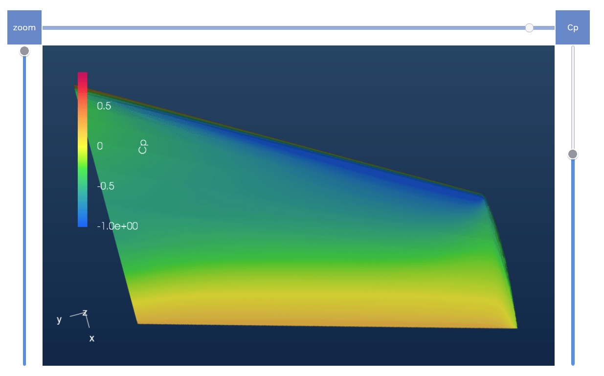
This tutorial will cover the case generator functionality of the Flow360 web client, used for specifying runtime parameters of simulations
Documentation
1.1. Run CFD using Web UI: An example of ONERA M6 Wing
Downloads
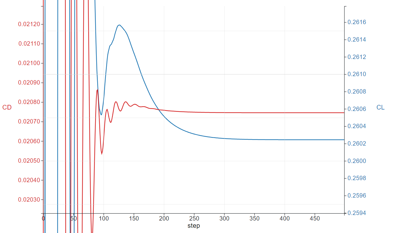
This tutorial will provide an overview of interfacing with the Flow360 client using the Python API
Documentation
1.2. Run CFD using Python API: An example of ONERA M6 Wing
Downloads
This tutorial will cover some of the basic features of the Flow360 web client
Documentation
1.1. Run CFD using Web UI: An example of ONERA M6 Wing
Downloads
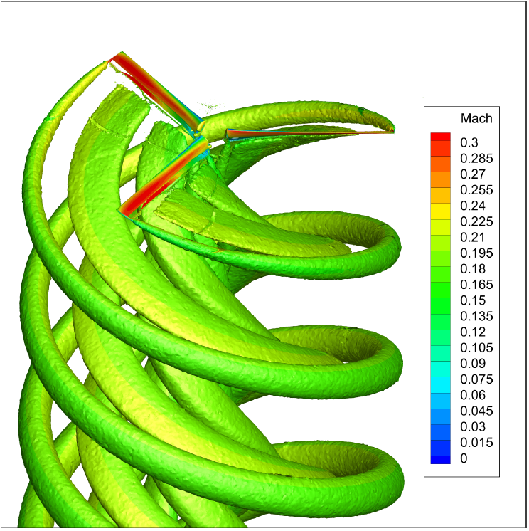
Flow360 can simulate a propeller using four different techniques, each with its own drawbacks and advantages. The goal of this article is to provide an introduction to each technique and give you the information needed to decide which technique is most appropriate for your simulation needs.
Four Different Propeller Simulation Techniques
1. Actuator Disk (AD)
The Actuator Disk technique is the easiest one to use in that all you need to give Flow360 is the thrust and torque distribution for your propeller. Flow360 takes that thrust and torque distribution and uses it to locally accelerate the flow. You can then see the downstream effects of the propeller’s thrust and how it affects the performance of whatever is downstream. The drawback is that AD can only be relied on if the flow is near perpendicular to the propeller disk. The AD technique assumes a uniform distribution of thrust along the azimuth. The thrust value and thrust distribution needs to come from another CFD simulation, momentum theory, experimental data or whatever other source you choose.

2. Steady-State Blade Element Theory (BET Disk)
When doing a steady-state BET simulation you provide a set of 2D polars as well as some geometry information representing the performance and shape of the propeller’s blades. That is, you provide a geometrical definition (chords and twists at many stations along the span of the blade) along with the 2D polars (lift and drag) at many slices along the span. The solver then uses that information to “build” a virtual blade in the flow. At each station the solver looks at the incoming flow, the defined geometry and its performance polar to calculate the forces that the blade would exert on the fluid and it applies those forces. The biggest advantage of BET over AD is that it is still accurate when the flow is not perpendicular to the propeller disk and it does not require you to know the thrust ahead of time like AD does.
Steady-state BET represents the propeller as a disk but it doesn’t mean that the thrust will be uniform along that disk. If the inflow is asymmetric then the BET effects will also be asymmetric. However, all time-dependent phenomena (e.g., tip vortices) will be averaged out.
To learn more about how and when to use the BET Disk model please visit this case study in our Flow360 documentation page.

3. Time-Accurate Blade Element Theory (BET Line)
The inputs to a time-accurate BET Line simulation are mostly the same as the steady-state BET Disk above. What is different is that you will now have your virtual blades spinning around and you will capture all the time-dependent effects. This, however, comes at the cost of much larger run times because the solver needs to simulate a lot of steady-state subiterations in order to come up with a time-accurate simulation over a relevant time span. The user should have an understanding of what sort of time scales the solution needs in order to capture the details of the flow physics while doing a long enough simulation to capture downstream effects of the propeller’s wake.

4. Time-Accurate Rotating Propeller (TARP)
This is the most computationally expensive technique, but also the most accurate. Here, you mesh the actual propeller geometry with hub and everything else and spin the propeller within a hockey puck like sliding interface. You can model multiple propellers each within their own sliding interface. You can model a sliding interface within a sliding interface to model various things like a helicopter’s cyclical blade oscillations. You can even spin things like a whole airplane to simulate aircraft stalling spins or model dynamic flight derivatives on entire configurations.
All the important flow physics are accurately captured (with a sufficiently resolved mesh). Not only can you have great trust in the resulting forces and moments, but you can also see how the wake from the propeller moves downstream and affects the various wings/bodies/etc. that are behind the propeller.

When to use which technique?
The choice of which technique to use depends on many factors:
- Do you have CAD for your propeller?
- Do you know the propeller’s 2D sectional lift and drag polars?
- Do you know the propeller’s performance (thrust/torque)?
- What is your flowfield like?
- Do you care about the forces and moments on the propeller, or the propeller’s effect on bodies downstream of it, or both?
- How much accuracy is required?
- How much effort/time do you want to spend simulating this case?
- …
If we go in order of simplicity:
-
Steady-state AD is best suited when all you have is the expected/desired thrust and torque values. The propeller doesn’t have to exist yet, for example, all you may know is that you need a certain amount of thrust and you want to see how that thrust will affect the flow downstream. Then AD is your best option as long as the inflow is perpendicular to your propeller disk (i.e., the thrust distribution is constant around the azimuth of the disk). One thing to note here is that if you change any of the simulation parameters (RPM, inflow speed, etc.), then you will most likely need to adjust the amount of thrust and torque your virtual propeller provides and you will need to know this from some other source (experimental, lower order methods, etc.).
Since it requires propeller performance ahead of time, the AD approach is only useful for scenarios when you want to learn how the propeller affects things downstream of it.
- Steady-state BET Disk is a very common option because most of the time you will know the 2D cross-section polars of your geometry. Once you have that information then you can simulate any scenario without having to change the propeller parameters. This makes running sweeps of any condition (alpha, air speed, RPM, etc.) very simple. You also don’t need to know the propeller’s performance ahead of time. With BET Disk you get both an idea of a propeller’s performance but also how it will affect things downstream of it. This is used a lot to test various propeller designs without having to CAD up each geometry variation which is very useful in the early design stages.
- Time-accurate BET Line is a lot more computer resource intensive then steady-state BET Disk, but it gives you a lot more information about how the blades behave in time. The most common scenario is if you know that you will have important time varying effects of vortices impinging on other bodies downstream, then you need time-accurate BET Line instead of steady-state BET Disk. Time-accurate BET Line gives you everything steady-state BET Disk does plus some information as to how things vary in time.
- Time-accurate rotating propeller (TARP) is your best choice if you have the CAD geometry and you need the highest accuracy possible. It is the most complex of all four techniques, but gives you the most accurate answers possible to all of your flow physics questions.
In any event, if you are still in doubt about which technique to use or have further questions. Please do not hesitate to reach out via support@flexcompute.com and we will get back to you very quickly.

Summary Table
| Technique | Pros | Cons | When to Use | Run Times |
|---|---|---|---|---|
| AD | Quick and simple | Only get information on objects downstream of propeller Can Only simulate normal inflow conditions |
When all you have is the propeller’s thrust and torque and your flow is normal to propeller disk | Very fast 1-10 (mins) |
| BET Disk | Quick and simple Very wide range of uses |
Requires accurate information about propeller’s 2D sectional performance | Most applications when you need quick turnaround with high precision and wide range of use cases | Fast 10-20 (mins) |
| BET Line | Same as BET disk but with additional time varying information | Same as BET Disk but with much longer run times | Same at BET Disk but time varying phenomena are captured | Longer 20-100 (mins) |
| TARP | Most accurate Captures all relevant flow physics |
Requires CAD geometry and high quality mesh Very resource intensive |
When nothing but the best will do | Longest 100-200 (mins) |
[1] Rotor5: Rotor analysis under 5 hours using ultra-fast and high-fidelity CFD simulation and automatic meshing
Rotor Analysis in Under 5 Hours Using Ultra Fast and High FIdelity CFD Simulation and Automatic Meshing
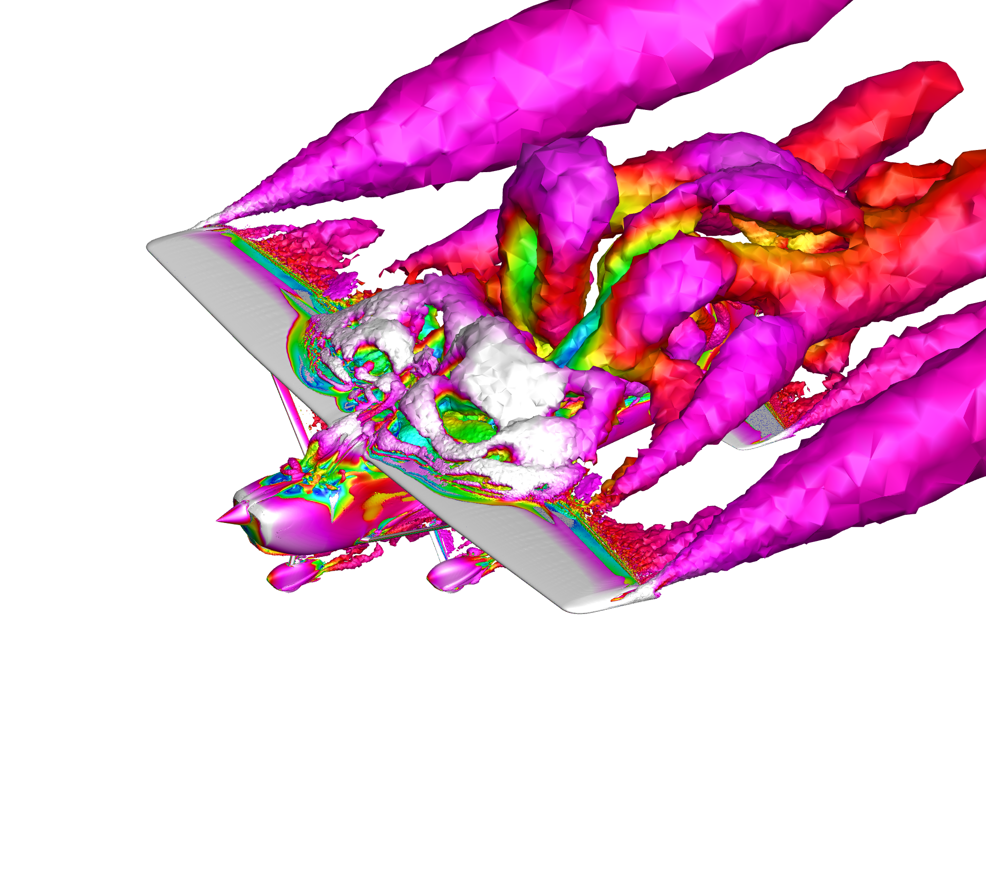
Pilots of fixed-wing aircraft receive training about how to avoid and, if needed, recover from aerodynamic stalls. A stall condition can result in a pilot’s inability to effectively control the aircraft, loss of control (LOC), and is a major safety concern[1]. Training involves intentionally maneuvering the aircraft to induce a stall under a variety of power settings and configurations.
The term “aerodynamic stall” or simply “stall” is used to describe a situation in which the airflow around the aircraft wings is no longer smoothly following the wing shape as intended. Specifically, flow above the wing separates away from the wing surface, causing relatively large regions of recirculating and turbulent flow. Separation, and thus stall, occurs as the angle of flow approaching the wing, angle-of-attack (AoA), increases beyond some design-specific threshold. A wing, or airfoil, will provide more lift as AoA is increased until the critical AoA is exceeded and stall occurs.
Figure 1 Coefficient of lift (CL) vs angle-of-attack (AoA) for a NACA 2412 airfoil.
While stall is directly related to the relative angle of the wing to the approaching flow, pilots are often provided with guidance regarding stall speeds of the aircraft instead. This is due in part to avoid reliance on sensors that measure AoA and also to relate to common flight operations, such as targeting an approach speed. Angle-of-attack is largely dependent on airspeed, however, so stall conditions can be avoided in practice by maintaining speeds above the aircraft’s stall speed. This AoA-airspeed dependence is the result of how much lift the wing is able to generate. The wing’s airfoil design determines the coefficient of lift, CL, vs AoA relationship as seen in Figure 1. This coefficient is nondimensional and is used to calculate the physical lift force. The physical lift force generated by the wing is proportional to the squared airspeed, U2, multiplied by CL.
What this means is that to maintain level flight (ie, lift equal to weight) at low airspeeds, the CL must be increased by increasing AoA. The slower the airspeed, the higher the AoA required and consequently, the wing moves closer to stall conditions.
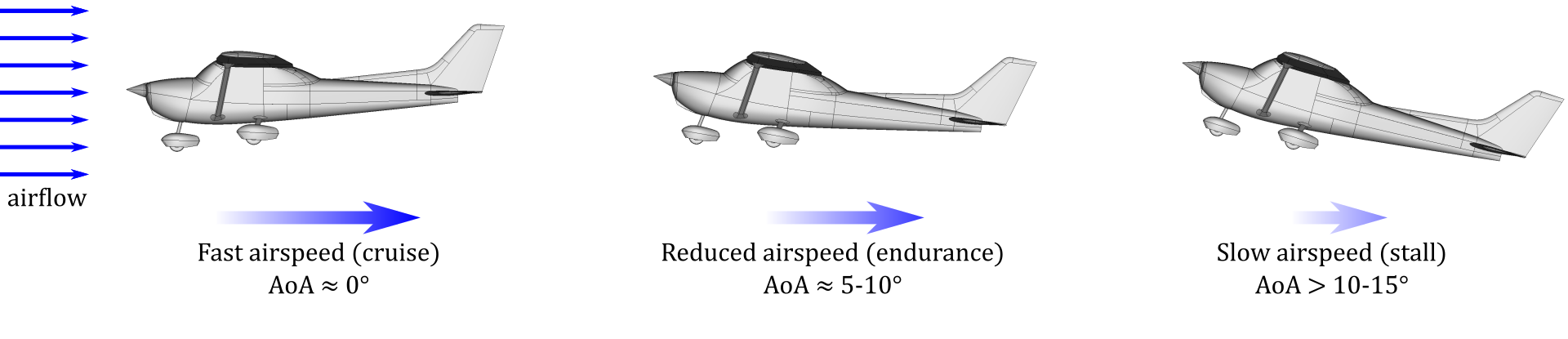
Figure 2 Angle-of-attack (AoA) relative to airspeed.
GENERAL CHARACTERISTICS
To investigate the details of aerodynamic stall, we use the Flow360 solver to create computational fluid dynamics (CFD) simulations of the flowfield around a Cessna 172 Skyhawk. Simulations consist of a simple AoA sweep, with smaller increments of AoA near stall.
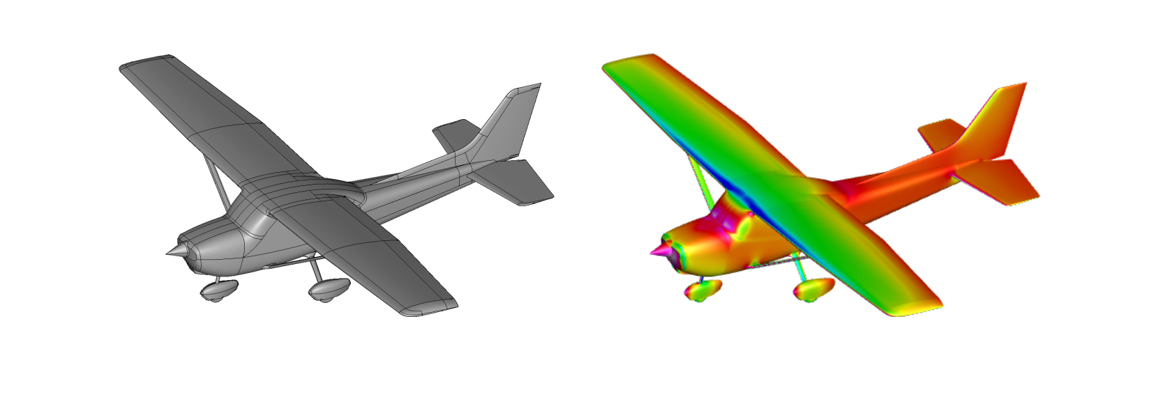
Figure 3 Cessna 172 Skyhawk geometry and pressure contours from CFD.
Creating a slice through the flowfield allows for a simplified view of the stall phenomenon. The following figures are slices at constant y (spanwise direction) and positioned at the mid-span of the port wing. Flow is from left to right. Pressure contours and streamtraces are displayed.
Results at AoA = 0° are consistent with classical examples of flow around an airfoil (see Figure 4). Streamtraces closely follow the airfoil shape everywhere. There is a strong pressure rise at the leading edge (LE) where incoming flow stagnates. Above the airfoil, a large region of low pressure is found along nearly the entire chord length.
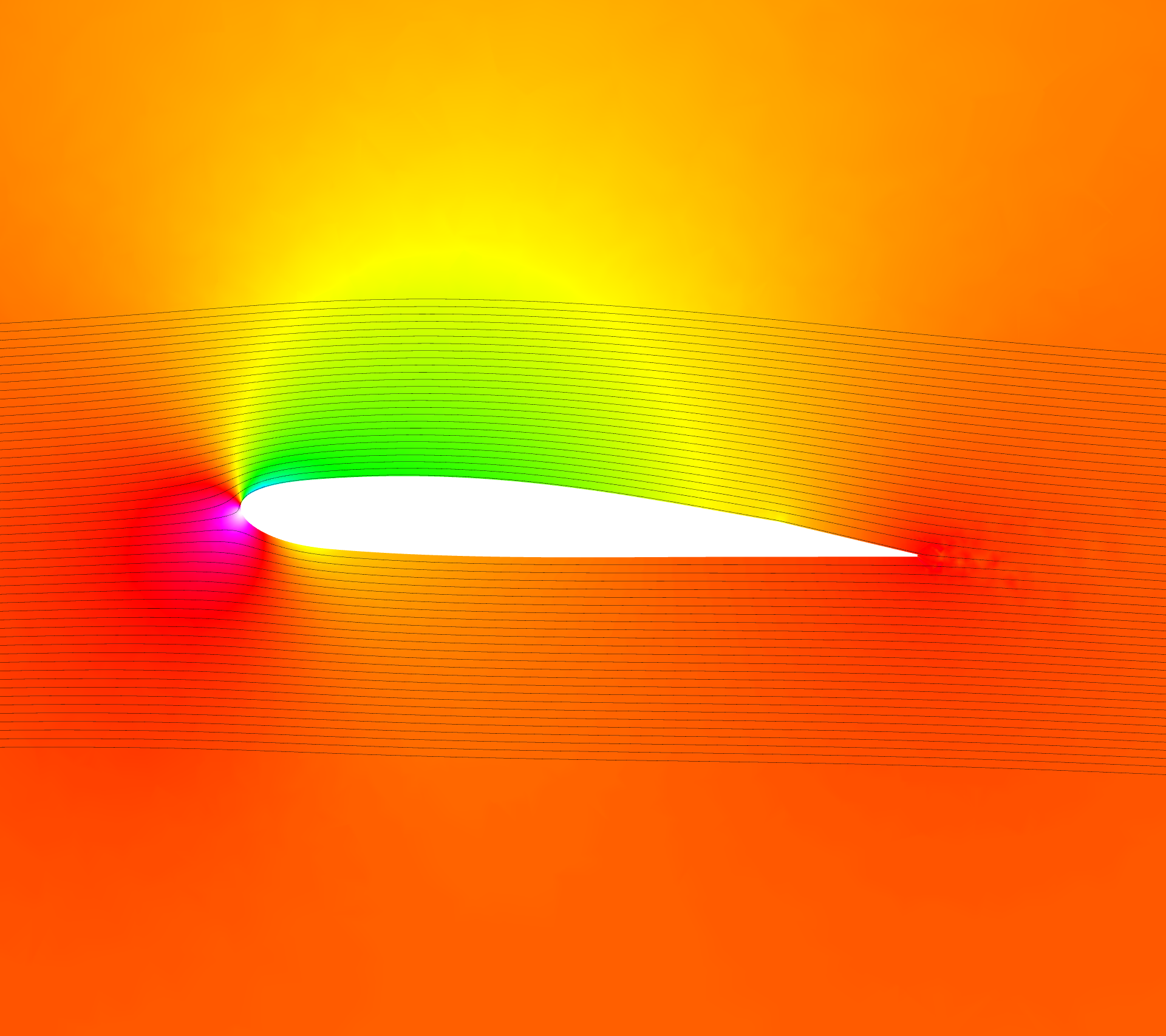
Figure 4 Slice through wing mid-span at AoA = 0°. Pressure contours and streamtraces displayed.
As AoA is increased, however, the flowfield changes significantly as stall conditions are approached (see Figure 5). At 10° AoA the upper low pressure region has increased in size and magnitude, which corresponds to increasing lift seen in Figure 1. Streamtraces still follow the airfoil shape as intended. As AoA is increased to 14° the initial onset of flow separation becomes apparent, indicating that stall is imminent. Following the streamtrace nearest the upper surface, at roughly ½-¾ chord the streamtrace noticeably deviates from the airfoil shape. Additionally, pressure contours at the trailing edge (TE) show fluctuations due to turbulence created by this separation region. Finally, flow separation envelopes the entire upper surface at 15° AoA. A large region of recirculating flow is prominent over the aft ½ of the airfoil. This dramatic change in the flowfield from 14° to 15° is indicative of aerodynamic stall, which can result in sudden degradation of aircraft performance and stability.
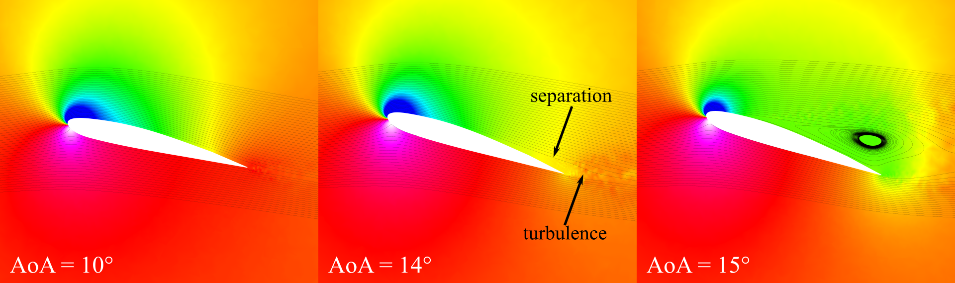
Figure 5 Progression of stall characteristics at increasing AoA.
ADDITIONAL FLOW PHENOMENA
Now that we’ve seen the basic flow phenomena associated with aerodynamic stall, let’s further investigate more complex features. The flowfield slices above essentially present two-dimensional steady-state flow around an airfoil. However, flow features around an aircraft approaching stall present many three-dimensional characteristics that are inherently transient. Aircraft stability can be severely impacted by these flowfield complexities that arise near stall conditions.
Visualizing surface streamlines (oil flow) on the upper wing highlights the localized effects of stall (see Figure 6). Contours of skin friction are also displayed where the presence of color indicates flow separation. The left figure at 14° AoA shows smooth flow in the streamwise direction along the outboard wing, but incoherent flow patterns inboard that indicate stall is imminent. Surface streamlines of the right figure at 15° AoA present four distinct recirculation patterns (stall cells) spanning most of the wing. The development of these flow features from inboard to outboard is a benefit of the C172 Skyhawk design; outboard control surfaces (ailerons) remain effective longer while approaching stall.
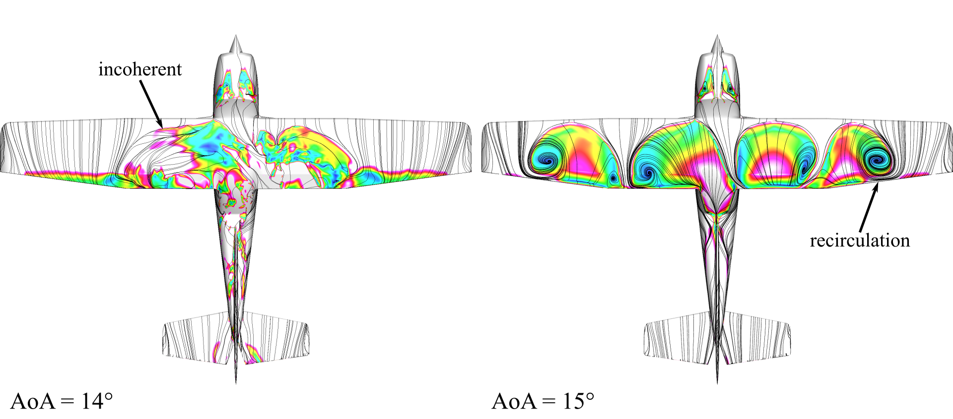
Figure 6 Top-down view of stall progression. Skin friction contours and surface streamlines displayed. The presence of color indicates flow separation.
As AoA approaches stall, these complex flow structures also vary in time. The video below displays the same surface streamlines and skin friction coefficient contours as above at 14° AoA. Local regions of separated flow move and change shape rapidly, inducing vibration of the aircraft and control instabilities. Additionally, asymmetric structures may lead to unintended roll and/or yaw of the aircraft which could further exacerbate the loss of control authority.
Figure 7 Transient behavior near stall. Regions of separation move and change shape rapidly.
Regions of separation, turbulence, and recirculation over a stalled wing are also not localized. Vortex structures propagate downstream of the wing and can directly impact aerodynamic characteristics at aft surfaces like the tail. Degradation of the horizontal and vertical stabilizers can potentially limit a pilot’s ability to recover from stall conditions.
Figure 8 Off-body flow structures. Iso-surfaces of Q-criterion colored by Mach contours displayed. Vortices propagate downstream and impact tail performance.
[1] Airplane Flying Handbook (FAA-H-8083-3B), Chapter 4.
FAA Airplane Flying Handbook
Despite a projected 40.3 million flights worldwide in 2020, airplanes actually have a major drawback. To take off, airplanes need to accelerate along a runway to reach the necessary speed to generate lift and become airborne. This limitation sparked the development of helicopters which use rotating rotor blades, instead of fixed-wings, to generate lift. This allows helicopters to take off and land vertically, removing the need for long runways.
However, helicopters come with their own restrictions which includes shorter ranges and slower speeds. Consequently, a new type of aircraft, the tiltrotor, was developed which combined the hover and vertical take-off and landing (VTOL) capabilities of helicopters with the speed and range of airplanes.
As the name suggests, tiltrotors utilise tilting rotor blades that are mounted to shafts at the end of fixed wings. During vertical flight, the plane of rotation of the rotors is horizontal, generating lift in a similar way to a helicopter. As the aircraft’s speed increases, the rotors progressively tilt forwards until the plane of rotation is vertical at cruising speeds. Here, the rotors act as propellors, providing thrust, while the fixed wings generate lift, just like an airplane.
The result is an aircraft which can switch between helicopter mode and airplane mode during flight, whilst achieving higher altitudes and greater speeds then a helicopter. These capabilities have attracted a huge amount of investment in the past and in the late 1960s, NASA together with Bell Helicopters developed the Bell XV-15 which has become the foundation for many VTOL aircrafts today.
Tiltrotor in CFD
To operate efficiently in both helicopter and airplane modes, the XV-15’s rotor blades feature complex geometry with high twist and solidity as well as a small rotor radius. This, along with the wide range of operating conditions makes it extremely difficult to accurately model tiltrotor rotor blades in CFD.
A few studies have been completed in the past which analysed the hover and airplane modes of the XV-15. These were based on full domain numerical simulations of the Navier Stokes equations. However, there has never been a comprehensive numerical study on the hover and propulsive/descending forward flight helicopter mode and airplane mode of a full-scale XV-15. To test the accuracy and performance of its Flow360 solver, Flexcompute decided to conduct such a study.
Model geometry
The XV-15 rotor is made up of three individual rotor blades, each consisting of five NACA 6-series aerofoil sections. The geometric properties of the full-scale XV-15 rotor were used to create the geometry file using the Engineering Sketch Pad.

Meshing
To accurately capture the behaviour of the airflows both around the aircraft and around the blades, a multiblock unstructured meshing approach was adopted. The entire domain was split into two blocks: 1) Farfield block acting as the stationary domain 2) Nearfield block acting as the rotational domain, containing the three rotor blades.
The farfield block (yellow) was designed large enough to ensure an independent solution with the boundary conditions employed. The nearfield block was merged by four components: a cylindrical off-body mesh and three cylindrical body-fitted meshes (orange) containing the blades (green). This allowed for CFD simulations to be completed over a range of blade collective angles from 0 to 18 degrees by regenerating the cylindrical body-fitted meshes perspectively.

The meshing process started with creating a cylindrical body-fitted mesh, which was then rotated along the axial direction to generate the other two body-fitted meshes. These were merged with the off-body mesh, with any overlapped nodes combined into a single node, resulting in one conforming mesh for the nearfield block.
The overall mesh consisted of a mixture of hexahedral, tetrahedron, prismatic and pyramidal cells to achieve the optimum balance between resolution and computational time. The mesh was further refined in particularly complex areas such as the viscous boundary layer near the blades which involved over 40 layers of hexahedral cells.

To model the rotating blades, the nearfield block will rotate within the stationary farfield block and so a sliding mesh interface needs to be solved. At each timestep, receiver nodes on the rotating mesh detect the two closest donor nodes on the stationary mesh. The receiver’s node’s solution is then linearly interpolated from the solutions of the two donor nodes and the process repeats for the next timestep.

CFD Results
The CFD simulations for this study used the Detached Eddy Simulations (DES) method together with Spalart Allmaras (SA) turbulence models. A range of results were analysed including overall and sectional blade loads, surface pressure coefficient, skin friction and the flowfield details. To validate the accuracy of the Flow360 solver, these results were compared with either previous CFD studies or experimental data from full-scale NASA wind tunnel tests where available.

Overall blade loads
The figure of merit (FoM) and torque coefficient (CQ) as functions of the thrust coefficient (CT) for hovering flight of helicopter mode were compared with three sets of experimental data. In both cases, the Flow360 results showed a strong correlation with wind tunnel measurements.

To analyse CQ and CT for forward flight helicopter mode, the shaft angle was varied to replicate a range of both propulsive and descending forward flight conditions. Compared to experimental data, the predicted rotor performance shows similar trends, but has a 4-14% relative error. Due to the lack of more precise pressure distribution and skin friction experimental data to validate these CFD results further, a grid resolution and time integration study will be completed in future to identify the reasons for these discrepancies.

For airplane mode, simulations were performed across a range of collective pitch angles and the results show good correlation with data from a previous CFD study and experimental data where available.

Pressure distribution results
To validate the predictive capabilities of Flow360 in capturing more detailed physics, the surface pressure distribution of the blades in hovering flight were also investigated. With no experimental data available, previous CFD studies using OVERFLOW2 and HMB3 codes were used for comparison.
Three radial stations were selected for the collective pitch angle of 10 degrees and the surface pressure coefficient (CP) was calculated based on the local rotating velocity at each radial station. In all three cases, the results from Flow360 align closely with the OVERFLOW2 and HMB3 results.

Overall, a detailed CFD study on the hovering and forward flight helicopter mode and airplane mode was conducted using Flow360 software from Flexcompute. After a thorough analysis and comparison with experimental data and previous CFD studies, Flow360 was proven to accurately predict the performance of the rotor blades in both hovering flight of helicopter mode and airplane mode. Further investigations will be conducted to fully validate Flow360’s potential to predict more detailed phenomena in forward flight helicopter mode.
For a deeper dive please refer to “Assessment of Detached Eddy Simulation and Sliding Mesh Interface in Predicting Tiltrotor Performance in Helicopter and Airplane Modes” in Flow360 Publications
It started in 2006 in Palo Alto, California. Like many graduate students, I woke up late in the morning, long after the clouds from the pacific ocean had dissipated. I would bike two miles across the Stanford campus and spend the rest of the day in the mezzanine of an old building with a lovely view of a quiet courtyard dotted by olive trees. Unlike the rest of Silicon Valley, things were slow here – at least to a graduate student working toward a Ph.D. in physics.
Things were about to get much slower.
My thesis was to develop silicon optical isolators. An isolator is a device that functions like a one-way valve for light. Without it, people could not fully leverage the power of modern semiconductor facilities to build next-generation optical communication chips. After working out some initial designs, it became clear that I needed massive computing power to validate those ideas. The computing involved solving large-scale Maxwell’s equations to simulate the physics of light propagating on a silicon chip. It required a megawatt supercomputer. However, there were not many megawatt computers in the entire world.
A long journey began. My Ph.D. advisor Shanhui Fan, who later became my co-founder, needed to convince the National Science Foundation to allow us to use one of their very few powerful supercomputers. He sent in a 5-page proposal. After a few months waiting, I got my password, delivered through postal service. The next step was to compile the code developed by previous Ph.D. students. I could smell the dust that the code had collected while stored in an external harddrive for years. Compiling it on a supercomputer was like reviving a roadkill squirrel. It took weeks before I could get it to work.
When I thought I was finally ready to conclude my study with just a few big simulations, it was actually the beginning of a two-year long effort. The computing jobs submitted to the supercomputer would wait for days or even weeks. As a result, I could only iterate my design once a week. It would be after 50 iterations and almost 2 years before I finalized an isolator design. Then I graduated with the work published as the cover story in a pretty good journal [1]. At the time, it didn’t bother me much that the speed of innovation was bottlenecked by a computer rather than by my brain power. While the productivity was painfully low, I took it as the cost of doing research.
Ten years later, in 2015, I was already an engineering professor at the University of Wisconsin in Madison. I relived the same experience again. The difference was that my graduate students would be patiently waiting for computing. This time, it really bothered me because it turned out that watching my graduate students waiting for computing is a totally different experience than waiting for computing myself as a graduate student. Ten years ago as a graduate student, I didn’t have to worry about the cost of payroll and a ticking tenure clock.
Later that year, I went to Boston to visit my longtime friend Qiqi Wang, an engineering professor at MIT who later became my co-founder. I was checking Instagram on my iPhone in an Uber when I had a sudden realization: none of these existed 10 years ago. Over time, business computing had brought innovations that made daily life more convenient – yet engineering computing had stagnated. We – the engineers who design new gadgets in the physical world– seemed to live in a world that had been forgotten by Silicon Valley entrepreneurs. We also need innovation in order to innovate faster! If no one would build new computing tools for us, we should roll up our sleeves and do it for ourselves.
Months later, Qiqi, Shanhui and I founded Flexcompute with one mission: using advanced computing to accelerate innovation. We were fortunately joined by a group of exceptionally talented friends who became Flexcompute’s early team.
Today, we are excited to announce that Flexcompute raises $22M in Series B funding led by Coatue Management with participation from additional investors. Proceeds will accelerate our efforts to build a world-class team and execute our vision of engineering computing.
Today, our computing technology is helping hundreds of university researchers from Yale, Purdue University, Columbia University, Boston University, University of Wisconsin, University of Illinois Urbana-Champaign, MIT, Stanford University and many other universities around the world. We are also proud to support dozens of companies to design their electric cars, electric aircrafts, high-efficiency wind turbines, and quantum computing chips. Simulating the physical world by solving massive differential equations allows them to design better and more efficient products. With Flexcompute they simulate an airplane in 5 minutes, instead of 10 hours before; a quantum circuit in 3 minutes, instead of 20 hours before. Our customers have never been able to iterate their designs so quickly. But this is just the beginning of a new era of engineering computing.
[1] Yu, Z., Fan, S. Complete optical isolation created by indirect interband photonic transitions. Nature Photon 3, 91–94 (2009).
We are thrilled to welcome renowned aerospace engineer Dr. Philippe Spalart as a Director of Fluid Sciences at Flexcompute. With his years of extensive experience, there is no one more qualified to head our fluid sciences.
Every engineer in aerospace in the last thirty years has heard Philippe’s name, largely thanks to his invention of the SA (Spalart-Allmaras) model in 1992, which has set a precedent across the aerospace community for advanced and accurate modeling with minimal complexity. Philippe’s contribution further extended much beyond aerospace engineering with the invention of Detached Eddy Simulation.
Philippe, The Spalart-Allmaras Model, and Detached Eddy Simulation
His love of engineering and aerospace started from a young age: he was interested in airplanes as a boy and later went on to finish his Bachelors in Engineering in France before emigrating to the United States with the intention of getting his Masters in Aerospace from Stanford. It wasn’t long before he was noticed and asked to complete his Ph.D. with the help of a scholarship from NASA. Needless to say, that was just the beginning of his career — both in aerospace engineering and in the United States.
“I came to the US for one year in 1978, and look what happened,” Philippe likes to say and looking back on his career, this decision moved Aerospace forward globally. He started at NASA with Direct Numerical Simulations, in which the turbulence is simulated without any empirical modeling before, in 1990, jumping all the way to the practice of modeling all the turbulence. His and his team’s work still encompasses the full spectrum, with aeroacoustics in addition.
His SA model was created to assist in the often frustrating process that comes with modeling the aerodynamics of the airflow around an airplane — a necessary part of designing every aircraft. The software and hardware available to us in the last decades had made predicting the performance of the airplane with the chaotic airflow traditionally difficult…to say the least. But what Philippe created was a model to heighten our understanding of this kind of turbulence flow, unusually with only one turbulence equation.
Everything we fly today, whether you take Boeing or Airbus, has probably been created to some extent with this very model.
Beyond the SA model, Philippe further increased the fidelity of turbulent flow simulation by hybridizing traditional turbulence modeling with Large Eddy Simulation, explicitly resolving those turbulent eddies not amenable to modeling. The resulting technique, namely Detached Eddy Simulation (DES) in 1997, is the most popular form of high-fidelity turbulent flow simulation used in various industries, including aerospace, automotive, and renewable energies. In 2017, Philippe was elected as a member of National Academy of Engineering for development and application of a broad array of computational techniques for the prediction of aerodynamic turbulence and noise.
Flexcompute’s partnership with Philippe has been a dream realized: his contribution will improve the accuracy within our newest endeavor to provide a timely and invaluable tool for the aerospace industry and beyond.
The SA Model and DES Combined With Flow360
Since their days studying at Stanford University, our founders yearned to see a more proficient method to achieve a faster resolution and to reduce the complexity of design. We’ve believed that more engineers and more aerospace companies should have access to use these models, like the SA model, in a timely manner, which is why we created Flow360, a flow solver built from scratch.
With Flow360, we’ve created a product that improves the computing speed by 100x. When designing an aircraft, usually it can take days or weeks to simulate the necessary conditions with any model. Using Flow360, any size or volume of cases can be completed in minutes or at most, within a few hours.
Philippe has said as much that this program was part of the draw to work with Flexcompute: “Flexcompute has the DES available, and makes simulations easier — recognizing the value of unsteady simulations — making it much faster and more financially feasible, and will predict the noise of this unsteady aircraft to help understand how loud the drone will be.”
“To paraphrase, running this unsteady simulation is necessary to understanding future safety problems,” one of our founders, Zongfu Yu says. “Running this unsteady simulation can be very expensive but Flexcompute provides the technology to simulate it much much faster at an affordable price, making it possible to study these facts with advanced modeling.”
With Flexcompute’s processing power, and Philippe’s proven history in modeling, these complex simulations and checks for safety via careful off-design simulations become a lot more accessible for other aerospace companies and even start-ups.
Predicting The Future of CFD
Philippe brings with him decades of first-hand experience to back him up on all things aerodynamics and beyond. His main concern, and ours, is accuracy.
“CFD is going to be a bigger and bigger part of engineering, for everything from modeling arteries to tornadoes, going through delivery drones like Amazon, cars, trucks, and wind turbines, planes, submarines… this direction is a lot better than it was 15, 10, or even 5 years ago… but it’s still not perfect,” Philippe emphasized.
In the industry, there are hundreds of startups emerging outside of Boeing, wanting to take drones to the next level to fly people and goods… creating larger versions of drones so they can carry more weight and be exceptionally safe. They desire a tight time to enter the market — they need to do it immediately and need a new set of tools to be the first ones to get there.
Philippe’s concern highlights our partnership’s focus: “CFD doesn’t ensure that physics will be correct. We don’t want things to just be faster, it needs to be accurate — if it’s flawed, then machine learning isn’t going to fix what you want it to fix. The 21st century will see more and more use of CFD, but we can’t just push a button.” It is a responsibility of the CFD provider to correctly represent the uncertainty attached to every turbulent-CFD approach to every problem, assuming the customer welcomes this partnership..
One of Flexcompute’s co-founders, Qiqi Wang, an associate professor of aeronautics and astronautics at the Massachusetts Institute of Technology, agrees strongly on Philippe’s view. “Flexcompute will benefit not only from his world-renowned expertise on turbulence modeling,” he said, “but also from Philippe’s broad knowledge in fluid mechanics and extensive industrial experience. These will help us build technology to help our customers achieve a much faster turnaround in their engineering design with state-of-the-art accuracy.”
Our Partnership
Combined with our Flow360 software, Philippe’s decades of experience with aerodynamics and simulations can elevate the internal expertise of all of our developers and customer-facing consultants. So his knowledge of physics with Flexcompute’s tech will help customers design their aircraft much more efficiently, and sometimes with lower risk.
Flexcompute is honored and proud to have someone of Philippe’s experience and knowledge join our rapidly growing organization. We are very excited for the impact he will have both for our organization and especially for our customers.
We strongly believe Philippe will continue to showcase Flexcompute’s dedication to adding the highest level of expertise to our team which, when combined with our record-setting technology, will provide Flexcompute’s customers with a level of value creation that no one else can deliver.
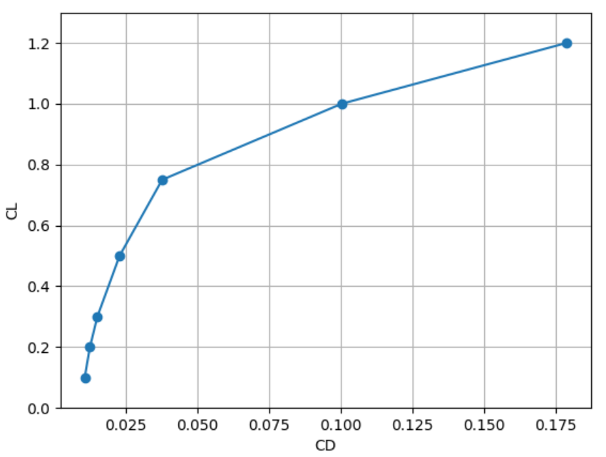
In this article, we describe how to run a speed sweep of an airplane using Flow360. A speed sweep analyzes the performance of the airplane when flying at different airspeeds while carrying the same load. Such analysis is useful for determining the most fuel efficient cruise speed, the optimal climb speeds (Vx and Vy), as well as the range of the airplane. This can be done in Flow360 in 15 minutes.
We start with the model airplane created using Xfoil and Engineering Sketch Pad (ESP), Meshed using Pointwise. The generated mesh is uploaded to the Flow360 web interface.
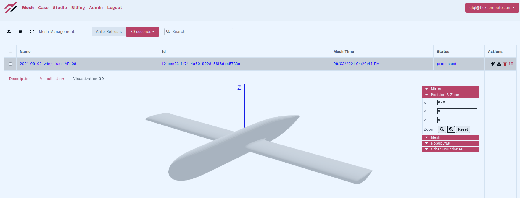
In the web interface, we fork a previous case of this mesh by clicking the “fork” button next to the case. Forking a case runs a new simulation that starts from the final solution of a previous case. This functionality is useful for continuing a previous simulation that did not have sufficient steps to converge. It is also useful for starting a new simulation with a slightly different configuration than the previous one. Forking is also used for continuing unsteady simulations.
For the speed sweep, we need to change the speed and target lift coefficient for each simulation. The speed can be modified in the “freestream”: “Mach” section of the input json file. The target lift coefficient can be found in the “runControl”: “targetCL” portion of the json input file. For a complete reference of the inputs of Flow360, please refer to our API reference at https://docs.flexcompute.com/api.html
Here, we set the lowest speed at Mach 0.158 and a lift coefficient of 1.2. Note that we set “startAlphaControlPseudoStep” to 1000, which tells Flow360 to start seeking for the target lift coefficient after 1000 iterations.
Once the case is started, the residual starts to be updated in the web interface. We observe that the convergence happens in two phases. The first phase happens within the first 1000 iterations, before Flow360 starts seeking the target lift coefficient. The second phase starts at the 1000th iteration, during which the target lift is achieved. We see that in slightly more than 4000 iterations, the target lift coefficient is achieved exactly.
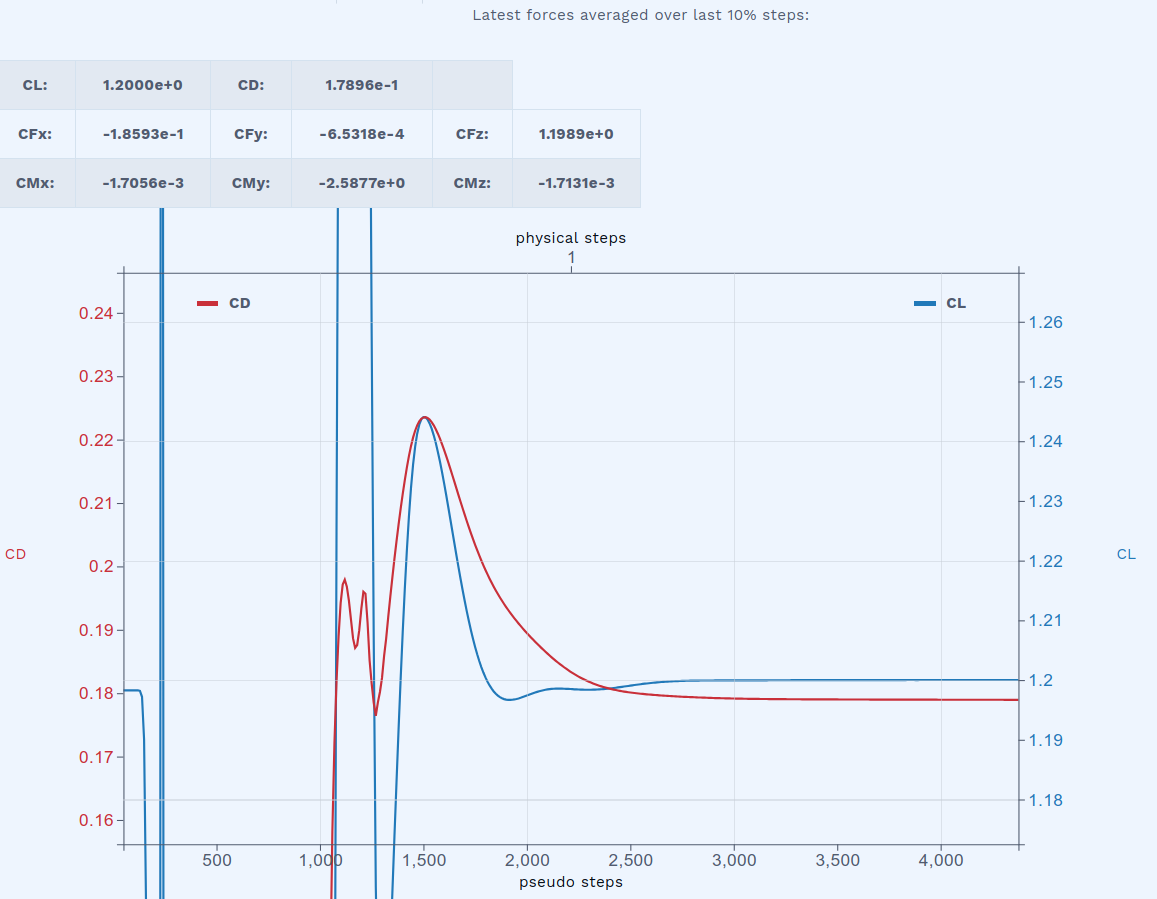
The aerodynamic moments are also updated during the simulation. Here, the x and z moments are almost exactly zero. The small values are due to the asymmetric mesh. The only significant moment is useful for determining the longitudinal stability of the airplane.
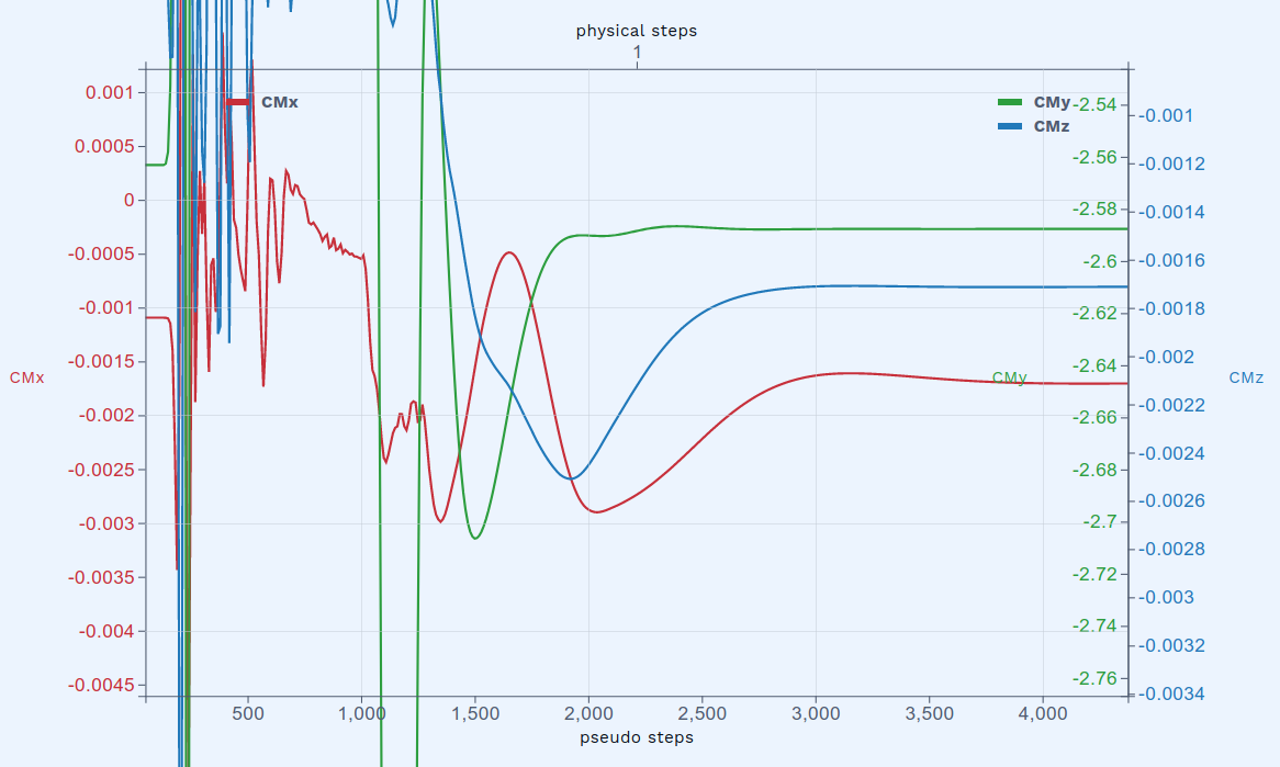
Also from the Flow360 web interface, you can examine minimum density, minimum pressure, as well as maximum velocity in the flow field, including their location. This is useful for identifying important flow features, as well as for troubleshooting diverging cases.
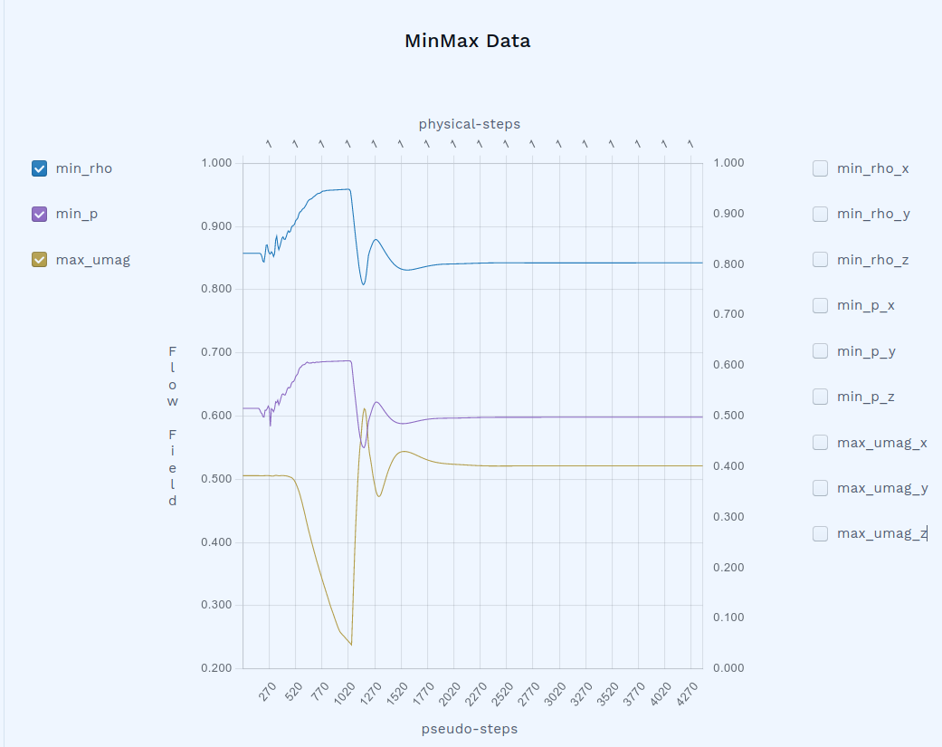
The speed sweep consists of a series of cases like this, at lift coefficients (CL) equal to 1.2, 1.0, 0.75, 0.5, 0.3, 0.2, and 0.1, respectively, each ensuring that the product of CL and the square of the Mach number is constant. Each of the seven cases, converging in about 4000 iterations on a mesh with 3 million nodes and 18 million cells, took about 2 minutes to complete. The entire speed sweep thus completed in slightly more than 15 minutes. After all the runs were completed, we obtain the following polar plot:
We observe that the drag coefficient increases roughly quadratically as the lift coefficient increases up to 0.75, and starts to increase significantly faster starting at a lift coefficient of 1.0. The lift to drag ratio, which determines fuel efficiency of the airplane, is also obtained. From this plot, we deduce an optimal cruising lift coefficient of 0.5, which produces the least drag for the weight of the airplane. Because drag is equal to the amount of energy required per flying distance, a lift coefficient of 0.5 means the optimal fuel economy.
The web interface of Flow360 also visualizes the surface flow path, colored by skin friction coefficient. Here shows the case for CL=0.1

CL=0.2:
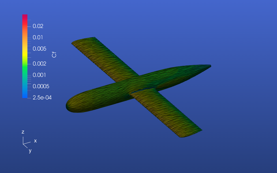
CL=0.3:

CL=0.5:

CL=0.75:
CL=1.0:
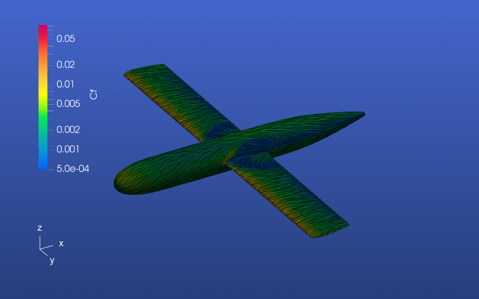
CL=1.2:
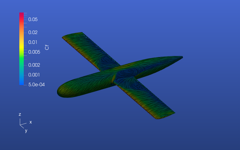
From these surface plots, we can deduce the reason for the significant drag rise starting at CL=1.0. The wing starts to stall from the root, which is typical for unswept wings or forward swept wings without significant wash-in.
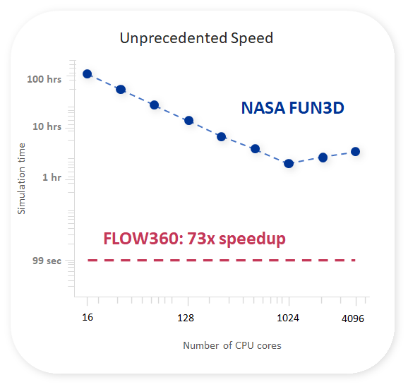
I am sure like many of you who are actively involved in Aerospace/Aviation CFD we are eager for the 4th AIAA CFD High Lift Prediction Workshop (HLPW-4) which is scheduled for January 7th in San Diego, CA. It has been over four years since the 3rd workshop (HLPW-3)! If you haven’t registered yet visit SCI TECH’s registration page for more information. For those coming from colder climates it certainly doesn’t hurt that the upcoming workshop is scheduled to be held in sunny San Diego… in January.
There is much to be excited about for HLPW-4 but what we are most excited for is the opportunity to put Flow360 on display against the most commonly used CFD solvers in the world. For those unfamiliar, after years of hard work and starting at the very foundation of what is theoretically possible for CFD solve speed on non-CPU hardware we launched Flow360 out of beta earlier this year. Flow360 is a co-design and co-delivered, cloud-based next-generation CFD solver that was written from scratch to maximize CFD solve speed on non-CPU hardware, including GPUs, TPUs and ASICs. It was still in the early development phase during the HLPW-3. We are now ready to show the world what Flow360 can do.
While we are hard at work preparing our results for the 4th AIAA CFD High Lift Prediction Workshop (HLPW-4) we wanted to look back at the 3rd workshop (HLPW-3) results and share with you all how Flow360 would have performed compared to the participants at the time. Benchmarking simulation in a true apples-to-apples fashion is always difficult and openly available models are often the most trustworthy. The HLPW-3 test case we executed was based on the high lift version of NASA’s Common Research Model. The stated goals of the HLPW-3 are below:
Objectives
- Assess the numerical prediction capability (meshing, numerics, turbulence modeling, high-performance computing requirements, etc.) of current-generation CFD technology/codes for swept, medium-to-high-aspect ratio wings for landing/take-off (high-lift) configurations.
- Develop practical modeling guidelines for CFD prediction of high-lift flow fields.
- Determine the elements of high-lift flow physics that are critical for modeling to enable the development of more accurate prediction methods and tools.
- Enhance CFD prediction capability for practical high-lift aerodynamic design and optimization.
Our results when compared to other CFD solvers amount to a game changer for the CFD industry. Flow360 was shown to be 73x faster (99 seconds compared to 7,227 seconds) than the fastest possible results of Fun3D which was run on 1024 CPU cores. For reference, this was the medium model which contained 27 million nodes and 46.8 million cells. It is also worth noting that many potential innovators do not have regular access to over 1000 CPUs for their CFD runs because, let’s face it, upfront cost and ongoing maintenance for on-premise clusters is extremely prohibitive for many companies and going to the Cloud DIY-style at this level of scale is nowhere near as easy as it should be. For these customers we can provide even more extreme speed increases. We have yet to see a steady-state run that we haven’t been able to solve in minutes, usually 10 or less, or an unsteady state run that we haven’t been able to solve in hours, usually 6 or less. Flow360 scales much more efficiently then CPU-based options and it automatically sizes the hardware configuration to the size of problem it is presented, hence the dashed line for Flow360 results instead of multiple data points in the comparison below.
While solve time is incredibly important because it enables innovators to test and iterate more options within a given deadline, above all else accuracy is of course of paramount importance. Flow360 was also a clear winner in terms of accuracy. As you can see below, Flow360 not only aligned extremely well with Fun3D and other commonly used solvers, but the results also produced with Flow360 at the coarsest mesh (8.3M nodes and 18.9M cells) better aligned with results from the finest mesh (208M nodes and 385.6M cells) then any other code. This unrivaled level of accuracy also enables users to not only solve at least 73x faster in an apples-to-apples mesh size, but it also enables users to get a consistent level of accuracy from smaller models, shrinking necessary solve times even further.
After achieving these results we knew Flow360 was ready to enable customers to dramatically drive down their design cycles times. Who should we first pursue with this record setting technology? Many companies could certainly benefit. We decided to target the eVTOL/eSTOL market where many pioneers are pushing the boundaries of what is possible with their innovative designs. We knew these companies would jump at the chance to adopt a tool that would enable them to reduce their time to market as it would provide out-sized returns in a hyper competitive space. One of our earliest adopters was Electra.aero, who is well on the path to pushing what is possible for sustainable regional mobility of people and cargo with their blown lift eSTOL design. Based on the results from our early collaboration, Chris Courtin, Lead Engineer of Flight Physics stated:
“Flow360 is a valuable tool for the Electra.aero team designing an electric short takeoff and landing (eSTOL) technology demonstrator aircraft. These aircraft depend on the strong interaction between the wings, flaps, and multiple propellers for high lift and flight control. Accurate simulation of many parameter combinations is required to develop insight about the physics of the problem, design the flight control system, and to evaluate the effectiveness of candidate design changes.
Flow360 provides an order of magnitude faster solution speeds and lower costs than our previous CFD solution, with no loss of accuracy. This enables an increased volume of simulation, which gives a deeper understanding of the aircraft across the design envelope. Critically, it allows us to react quickly to the results of these studies. Our time required to iterate design changes from multiple weeks to a few days with Flow360. This was a very significant time savings on a compressed project schedule.
With a small team, we also benefit from the easily scalable and turn-key nature of the Flow360 system. It gives access to state-of-the-art results, without the overhead of maintaining a large dedicated CFD group. The pace of the simulations can be easily scaled to match the current needs of the project.
This combination of rapid, high-quality results with a system that can flexibly adapt to project needs is what makes Flow360 such a compelling product.”
Fast forward 9 months and we are quickly becoming the tool of choice for the leaders in the advanced air mobility space and count many, including a majority of the top 5, from the AAM Reality index as customers.
We are eager to present our formal results for the upcoming HLPW-4 and expect Flow360’s results to again stand well above the field in terms of speed and accuracy.
You can see more of Flow360’s results from the HLPW-3 on our documentation site.
We would like to hear from you! The speed increase and efficiencies gained with Flow360 effectively open up the range of aircraft design problems that can be tackled with CFD. If there are problems that you previously thought were too large and complex to solve in an acceptable timeframe or you would like to benchmark your current CFD solver/hardware setup against Flow360’s co-delivered, browser-based, cloud-delivered platform, or would simply like to learn more reach out to support @ flexcompute.com
Thank you for reading, we look forward to seeing you all in San Diego next January!
In this article, we illustrate a typical workflow of using XFoil, Engineering Sketch Pad (ESP), Pointwise, and Flow360 to analyze the aerodynamic performance of a wing-body configuration. The goal is to perform RANS simulations of several airplane models, each with a wing and a fuselage, and to compute the drag and induced flow downstream of the airplanes. In less than half an hour, one can go from a pure concept to concrete CFD solutions, with outputs ranging from key quantities of interest to surface pressure and streamlines, and to detailed three-dimensional flow fields.
The process starts with two-dimensional design with Xfoil, which takes 5 minutes with some familiarity with Xfoil. It then proceeds to the construction of a three dimensional model, which also takes 5 minutes if one is proficient with ESP. The next step in the process is meshing, which takes about 5 minutes of human time – no geometry cleanup required – and another 3 minutes of computer time. Finally, uploading the mesh and running the simulation with Flow360 can take less than 5 minutes with a good Internet connection and familiarity with the Flow360 web UI.
The first step is to design the airfoil used in the wing and the fuselage geometry. Here we use the NACA 0012 airfoil for the wing. We extend the maximum thickness of a NACA 0024 airfoil horizontally to make the fuselage shape, as shown below. For how to use the open source software XFoil to design airfoils, please refer to its documentation at XFoil Subsonic Airfoil Development System


The next step is to construct a three-dimensional geometry using Engineering Sketch Pad (ESP). We used the REVOLVE command to make the fuselage from the two-dimensional cross section, Each airfoil section is scaled and translated into its respective position. Note that we extended the chord around the wing-fuselage junction, a simple method to reduce junction flow separation. The smooth airfoil is split into upper and lower surfaces, each represented using a SPLINE. The blunt trailing edge is represented by a line segment. The resulting series of closed contours are formed into a half-wing using the BLEND command. The other half wing is then constructed using the MIRROR command. The fuselage and both wings are then joined into an airplane using the UNION command. For how to use ESP to construct 3D models, please refer to the examples and documentation at Engineering Sketch Pad (ESP)

The resulting model is saved into an EGADS file and imported into Pointwise. Typically, no geometry clean-up is necessary with the EGADS format. We then use Flashpoint, an automatic surface generation tool, to generate the surface mesh. We set the maximum aspect ratio to 50 and turn refinement off at concave edges to obtain good mesh around trailing edges. For more information on the Flashpoint feature of Pointwise, please refer to Mesh and Run a High-Fidelity Aircraft Simulation in Minutes

To generate the volume mesh, we first create a spherical mesh with a radius 100 times the length of the airplane. This spherical mesh serves as the far-field. We then create a block in the space between the far-field mesh and the airplane surface mesh. We add a box-shaped source behind the wing to resolve the induced flow. Volume mesh is then generated using the TRex algorithm, the first layer thickness on the wall set to one-millionth the length of the airplane. Before saving the mesh into the CGNS format, we name the airplane and far-field with different boundary conditions. For more information on how to use Pointwise, please refer to Pointwise

We then upload the mesh to the Flow360 website. After the mesh is processed, we see on the webpage that the mesh contains about 2.4 million nodes and about 14.5 million tetrahedrons. In the visualization tab, we confirm the correct mesh is uploaded by inspecting the surfaces.


We then launch a Flow360 case from the mesh. We specify a Mach number of 0.3, a Reynolds number of about ten million, and a target lift coefficient of 0.5. The simulation converged in slightly more than one minute. It took over two thousand steps to converge the mass conservation, momentum conservation, and energy conservation equations to the default tolerance 1E-10. It is worth noting that the angle of attack is automatically adjusted starting from the 1000th iteration in order to match the target lift coefficient of 0.5. For more information about how to set up a simulation in Flow360, please refer to Flow360 Documentation

The convergence history of the lift and drag coefficients can also be observed from the Flow360 website, both during the simulation and after it completes. We see that the lift reaches the target of 0.5, and the drag coefficient converges to 0.0268. The convergence of other forces and moments is also displayed.

After the simulation completes, we can inspect the surface flow field by clicking the visualization tab on the Flow360 website. The surface streamlines show attached flow both on the wing and on the fuselage.

The pressure coefficient can also be visualized on the webpage.

The above workflow can be easily automated by simple scripting. We use such automation to build, mesh, and simulate several airplanes of different aspect ratios: 3, 5, and 8. The pictures above correspond to an aspect ratio of 8. The following pictures show the web-based pressure coefficient visualization for the lower aspect ratios, with the same nominal wing area.


To examine more details of the simulation, we can click the “download” button on each completed case for the visualization files, available in Tecplot and Paraview formats. These files contain the entire flow field. The following figures show the Z-velocity on a plane 20% airplane lengths after the tail. For more information about using Tecplot for flow visualization, please refer to Tecplot


The wingtip vortices and induced flow are clearly visible. Although the three airplanes generate identical lift forces, the tip vortices and induced flow are clearly stronger for the lower aspect ratio wings. This is reflected in the drag coefficients. All three airplanes achieve the same lift coefficient of 0.5 with identical reference areas. The drag coefficients computed by Flow360 are 2.6815e-2, 3.2031e-2, and 4.1975e-2, respectively, for the airplanes of decreasing aspect ratios.
The entire process from concept to CFD solution takes less than half an hour for a proficient engineer, and much less than that if the components are automated by scripting, which is supported in ESP, Pointwise, and Flow360. Such a fast and automatable workflow can dramatically accelerate the design iteration cycle of your aerospace vehicles.
SUBSCRIBE TO RECEIVE
UPDATES
Stay up-to-date with the latest news and thought leadership in
multiphysics simulation technology.